Blog Post 6: Data Collection

As previously discussed in Blog post 5, and small assignment 2, I collected data to help me understand the factors that influence the growth of bean plants specifically as observed at Duggan Community Garden. The hypothesis of my research is to determine whether the presence of other plants growing near an individual bean plant influences its growth and abundance; and therefore, due to greater plant diversity in garden plots reducing intra-specific competitions which would result in larger bean plants.

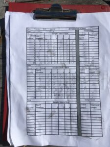
In this module, I completed all my data collection. I gathered data was from two different locations, which represents two different garden beds. Each garden bed area was about 5.56m2, 3.81 length, and 1.50m width. For both locations, I did 10 sample replicates. Each of the 10 sample units was 30cm away from the others to allow for independence of every single one of them.

One of the problems I faced, was that I was unable to collect data from the third location, as I had initially planned to do so. This was because of the inaccessible fence around this garden bed, I could not reach individual beans without making damage. Therefore, I decided to avoid any damage, and thus just collected data from only two locations.

The patterns observed have made me reflect on my hypothesis. I would not say that there is significance between the abundance of bean plants and the number of other types of plants growing nearby, but the data show a potential correlation. Also, I think my data is not sufficient to determine the significance of this relationship. However, I believe that I will be able to come up with a more developed conclusion once I analyze my data on a more detailed and deeper level, and when I read more literature about similar research.

Blog Post 6: Data Collection

For my research project, I am collecting data on soil moisture to see how it affects the distribution of Cedar trees. I am also collecting extra data on moss biomass. To do this, I am using 0.5 m2 quadrats randomly placed in both sites with Cedar trees and sites that have other trees but no Cedar trees. My data collection is ongoing at this point. I have so far collected nine moss samples from sites without Cedar trees, eight moss samples from sites with Cedar trees. My goal is to collect ten samples from each site type. Moss sampling has been going on without any problems since I fixed the GPS problem discussed in blog post five.

My biggest problem implementing the soil sample portion of my project so far has been finding the time to do it. I am aware that soil moisture varies on a day to day basis, especially with the intermittent rain that comes with spring in Nanaimo, so I must collect all my samples in one go. My plan is to collect 20 soil samples (10 for each type of site) so I know I will have to block off an entire day to do this. I will spend a day this weekend to get it done.

Since my hypothesis has changed to the effects of soil moisture on Cedar tree distribution, moss biomass has become my ancillary pattern. It seems that there is more moss in areas where I predict there will be less soil moisture. This doesn’t make sense to me, as moss tends to grow best in moist areas. This may mean there are other influences here that I am missing.

Update: I have now taken all my soil samples. The only problem I ran into was that I couldn’t dig very far down, as there were too many rocks, so all of my samples are from the surface. Other than that, I successfully collected all my samples before it began to rain!

Blog Post 6: Data Collection

Data collection for my project is ongoing. I am observing if the abundance of snow fleas seen on the surface of the snow changes under open or shaded circumstances. My prediction was that snow flea abundance would increase under shade.

I decided to keep on with the same data collection strategy that I used during my initial data collection venture but to ramp it up with multiple observations/counts over several days. Five 0.5m2 treatment quadrats (located under a shaded structure) and five 0.5m2 control quadrats (fully exposed to the sky), randomly spaced in a section of garden, have been visited 3 times a day since March 19 with the goal to continue this systematic temporal observation process until at least March 23. That will make a total of 15 observations, five at 10:00, five at 13:00, and five at 16:00 over the course of five days, to see if a pattern of snow flea preference to open or covered sites is apparent. So spatially there are five treatment and five control replicates, with data measurements occurring 15 times.

So far, the data collection process is going well. I have created a better data collection sheet (Figure 1) and have streamlined the process of collection so that each each count goes relatively fast. Some of the measures I took to facilitate counting should snow flea numbers be too high to quantify in 0.5m2 quadrats have been seemingly unnecessary – though I continue to divide each quadrat into 10cm x 10cm subsamples and quantify snow flea density inside each.

Even though I believe that my hypothesis is worth investigating, I’m finding that my prediction is a bit off base and that snow flea abundance appears to be greater in the open. Other weather-related factors such as cloud cover, precipitation, wind intensity, and changes in snow quality as a result of the artificial shade may be contributing to observed patterns as well as my original prediction which was based on naturally occurring shade within forests. Snow flea abundance has not been as great during this time as I had hoped, and I plan to keep the study site set up even after these 5 days are over so that I can continue to observe snow flea presence and abundance under open and shaded treatments, especially if their surface numbers explode under the right environmental conditions – factors which are still a mystery to me.

Figure 1: Updated data collection sheet

Blog Post 6: Data Collection

My research project looks at the expansion of a stand of Trembling Aspen Populus tremuloides into a field at Campbell Valley Park in southwestern BC. I chose to sample using transects along 2 randomly drawn locations along the field started from the side of the stand. With 5 sampling points along the transects and trees sampled in each “quadrant”, I took 40 replicate samples. The sampling was fairly straight forward, but I did not expect to be caught up in so may dried blackberry bushes!

I originally chose this location last year when the leaves were on the trees and the forest was dense. I have now gone back to do my sampling and the forest and trees look much different in the winter. The soil was dry then and now it was very moist and even saturated in some sampling points. Since the forest was also bare, I could see different patterns that were not as clear in the winter. While I still think the Aspen are growing into the field, since this is the only location where the stand can expand (the back is paved and there is a trail to one side), there may be more environmental drivers behind this. I will now have to look at my data and see if my hypothesis of a higher density of younger trees near the forest edge is shown.

Blog Post 6: Data Collection

For my data collection I used transects as a sample unit and 1×1 foot quadrants as my subunit.  I had 10 replicates of each sample.  Each transect was 10 meters apart and each began at the edge of the foot path, followed the gradient down the mound of the hilling and ended in the peatland.  The transect was interrupted at 5 m intervals.

I did struggle implementing my design a little because it was harder than I expected to walk that far off the pathway and into the peatland area.  I also ran into a little more soil water-logging than I had expected but that may be due to the time of year I took these samples.  I used an EXTECH pH Module to take the pH from the centre of each quadrant.  It was a little difficult walking through the peatland with all my supplies and taking the pH sample from the centre of each quadrant.  Some of the quadrants had large plants in the middle that I had to work around to reach the soil below. 

I will be reflecting on the water moisture, pH, and soil composition.  I also might think that there is something to be said for how hard it was to walk in there and so how less disturbed it must be by humans overall. 

Post 6: Data Collection

Field data was completed today. In total there are 30 replicates with 10 replicates of each condition. One of the issues that arose was that a few of the fronds sampled were eaten by insects or animals and so were shorter than expected. When processing data, these frond measurements will be excluded as they were shorter due to factors other than the amount of sunlight. Another problem I encountered was that it was exceedingly difficult to balance my lab notebook and measuring tape and so I acquired the help of a friend to record the measurements as I read them aloud. A third issue I encountered was trying to avoid stepping on other flora when walking towards and measuring the ferns. Otherwise, the data collection went relatively as indicated in my experimental design. The refinement made during the initial sampling was very helpful in making this process smooth.

One trend I noticed was that the eaten ferns tended to be in the shade treatment. While this does not change my hypothesis or alter it in any way, it is interesting and likely a result of the fact that the plants prefer the dense forest to sunlit urban backyards. Another factor I noticed is that the temperature is cooler in the woods than in the sunlight and I wondered if this was a factor in fern growth. Lastly, I noticed that in the shaded area there are a lot of plants and fungus including ferns, moss, trees, lichen, and other plants whereas in the semi-shaded area there was less variety of plant life as much of it lives on the edge of human activities. The sun area appeared to have a greater variety of grasses and other leafy green plants as opposed to the trees, moss, ferns, and lichen of the shaded forest. This does not change my hypothesis, but could potentially be a factor in accounting for the differences between the treatments.


Blog Post 6: Data Collection

First day of sampling occurred on Saturday, Feb 27th at approximately 9:30am within the headland island of Pipers Lagoon, in Nanaimo B.C. 

Study Hypothesis: Broadleaf Stonecrop abundance is determined by substrate drainability.

For my first day, I sampled three replicates on the Western portion, and one replicate on the Northern portion of the headland island. Each replicate consisted of a 40m long transect with the starting point randomly placed above the high water mark along the backshore. I originally planned to do a 50m length but felt it was redundant to sample that far into the inland forest. I chose the heading of each transect to be approximately towards the center of the headland island. Each transect, therefore, covered the full environmental gradient from coast to inland forest.

Along each transect, I placed a 1m2 quadrat starting at 0m and then every 3m, for a total of 14 subsamples per transect. Within each quadrat, I recorded the elevation above sea level, the substrate type, the sloping characteristic (gradient), the percent cover of my study subject (Broadleaf Stonecrop), and the distance along the transect. I also made note of the amount of sun exposure specifically whether it was an open space, or shaded by other vegetation.

Overall my study design was effective, albeit somewhat time-consuming. To speed things up a bit I may take pictures of each quadrat and from those assess the percent abundance and substrate type. I did have to adjust the starting locations of a couple transects slightly to allow for safer access to points along the transect.

Generally, my data collected thus far does tend to agree with my hypothesis, although based on patterns observed, sun exposure does seem to also play an important role in the Broadleaf Stonecrop abundance.

I will continue to implement this study design throughout the remaining area of the headland island. This will require 2 more transects in the Northern portion and 3 each in the Eastern and Southern portions for a total of 12 transects (replicates).

Post 6: Data Collection

Because the natural park that I was sampling from is located almost directly next to my place of work, I was able to sample each morning for an hour before heading to work. I sampled from 7-8am each week day starting from January 11th, until February 5th. This meant that I sampled on 20 separate occasions. It was made extremely easy in that it is so close to my work place. With my markers set up for my three testing locations, I spend twenty minutes at each location observing the bird species that I see. I created a tally sheet including any species that have already been identified, with room for any new varieties. Sampling at the location itself went quite well and was relatively easy. Some mornings were quite cold, but it was interesting to observe how different weather conditions seemed to influence the presence of bird species. There were species which I was unable to identify. In those cases, I would take a few pictures of the bird and then identify at a later time. That was challenging at times, thought with the resources I have and the expertise of the staff on site at the natural park, I was able to identify all birds that were observed. The ancillary patterns which I observed did not consistently support my hypothesis. Other considerations such as temperature, precipitation, and hiker presence seemed to contribute to the presence or lack or presence of bird species variety and abundance.

Blog Post 6: Data Collection

Hypothesis:

The level of predator activity in an area does not affect the activity of a mole colony in the same area.”

Field Data Collection Activity:

Field data related to mole colonies and predators continues as I refine the process by which to conduct the collection. Originally I had intended on selecting a set mole colony inside of the Western Ukraine Research Area (WURA). However, the grid layout and detailed counts became unwieldy as I noted that the feral dogs would intrude during the longer time taken to gather data.

I altered my plan by researching point counts and how to conduct them in order to capture accurate information. Included in this process I laid out a routine path along which I will be conducting my data gathering. This consistency will improve the accuracy of my data.

Already I have tested this out and am using 10 replicates along a sampling route in the WURA. The intention is to do this for the next ten days in order to get the magnitude of data needed for a statistically relevant study. There will be ten repeats of the sampling process giving us 100 samples to work with.

Initial survey results show that there may be a correlation between predator activity and prey (mole) activity, but more data is required as ‘correlation does not imply causation’, especially in such a small sample count. It would be easy to jump to a biased conclusion before the data is completed.

Another alteration to my plan, is to identify the mole colonies as individual colonies rather than the zone identifications. Some colonies are in the same zones, so I will be labeling them as their own independent colony moving forward.

I am excited to continue the research project as I feel I now have an effective sampling method and there is a great deal of confidence that it will work well for what I need.

Fig. 1. Sampling path

Post 6: Data Collection

I would have liked to be able to get further into the forest for at least some of my sample areas but the season and level of snow made that option unavailable. Sampling trees that do not have human interference in their immediate environment would help minimize the impact of some confounding variables. I chose the trees using the haphazard technique and sampled at least three replicates in each area. In total I sampled trees from five different and distinct locations in the local area. I did notice that the results seemed to be dependent on more than just the direction of the sun. It seems other factors could be influencing the location of the green color. It could be that there are more variables than I originally thought. I hope to find some other possible explanations after compiling all the observations.