I collected my data from two different transects. One located on Elbow River in Kananaskis, AB, the other from Ing’s Mine- across the highway from Elbow River. The Elbow River transect is located on a steep South-West facing slope with no canopy or other forest cover. The Ing’s Mine site is well shaded with a medium density canopy and underbrush. At each transect five separate kinnikinnick plants were randomly selected. There were four separate branches/trails from each selected plant that were measured for length of branch in inches. The Elbow River was measured in absence of canopy with direct sunlight where as the Ing’s Mine site was measured with presence of canopy with indirect sunlight. One problem that occurred with implementing my sample design was finding Kinnikinnick plants at the Ing’s Mine site that were not encroaching on each other (patchy distribution found under the canopy). A pattern found at the Elbow River transect was that the branch lengths were commonly around 22″ and the Ing’s Mine transect they were commonly around 7.5″. These patterns help show on a very small scale research site that my hypothesis: Forest canopy will negatively affect the growth rate of Kinnikinnick (Arctostaphylos uva-ursi) has potential proof.
Category: Post 6: Data Collection
Blog Post 6: Data Collection
To date I have gone out twice to collect field data at my grasslands site in Vernon BC. To this point I have sampled ten replicates. Each replicate is a different transect line along a slope gradient from a gentle lower slope position to a steep mid to upper slope position. On each replicate I have sampled 4 plots, totalling 40 plots. I have not had any particular difficulties implementing my sampling design.
A point of observation that I made on September 26th, on my second data collection day was that soil samples on the lower slopes demonstrated hydrophobic reactions to the water I added in conducting the texture analysis. I did not notice this pattern with the soil on the steeper slope position. This will be a point of further research into soil property characteristics.
I have not noticed ancillary patterns, however I have noticed that the vegetation has a quite a distinct zonation between gentle and steep slope sections, with predominately grasses on the gentle slope and forbs/shrubs on the steep slope section.
Post 6: Ongoing Observations
So far, my data collection has been going relatively well. The methods are easy to implement and I don’t have many physical obstacles that could hinder my study area. Zonation gradient does not seem to influence ant absence/presence as I found them in each ecotone, and elevation is not a factor to consider in my study because it is too minimal across the study site.
I am, however, finding that my data does not seem to fully confirm or support my hypothesis, as many factors affect patterns that I am to observe, and this will need to be addressed in the discussion of my research.
Some of these factors are:
- My predictor variables are not as straight forward as I anticipated; while vegetation cover could potentially affect ant presence, I found that it was most difficult to observe presence/absence in 100% vegetation cover of my quadrats. Additionally, disturbance was an issue and this was a significant flag when I noticed that pocket gophers created mounds of dirt of which were mostly present in the most vegetated zones, creating discontinuity. This type of disturbance favored my hypothesis only because the uplift of soil above the vegetation enables ant activity and exposure.
- Precipitation is a factor that affects soil moisture (another predictor variable), however, the issue here isn’t the soil moisture as much as it is the daily precipitation, where they are not seen.
- Another climate factor is temperature. As it is getting closer to “hibernation’ where ants start to slow down biological function, this phenological timing will affect my future findings. This might become another factor to consider in my data collection.
- Lastly, The goal of my study is to identify if there is a correlation with ant habitat preference on an environmental gradient. Certainly, ant species behave differently, and hopefully this will not cause a fundamental flaw in my overall hypothesis.
Blog Post 6 Data Collection
I collected my field data on 2 separate days (March 4, 2020, and August 6, 2020). The second survey day was to address my initial field survey design flaws. I needed to replace my dropped eastern auxiliary plot (as the original had been in Lost Lake) and to collect 5 more replicates. I increased the number of replicates, as 10 is the oft-repeated rule of thumb for a variable of interest.
As I now have 10 replicates, and 4 trees surveyed at each replicate, I have 40 trees sampled. I used the Vegetation Resources Inventory (VRI) Ground Sampling Procedures methodology to replace my dropped auxiliary plot. I also used these methods for 5 additional replicates, totalling 10.
August 6th was overcast, 20 degrees Celsius and called for rain. It had rained in the morning and I had hoped to collect data within the opening that rained ceased in the afternoon. I was unlucky and I had also not made my data sheets on water-proof paper. It was really difficult and an oversight I would never do again.
In my hypothesis, I stated that I would find conks on only one tree species and that is currently not being supported by my data. I have found conks on deciduous and coniferous trees. What is being supported is that conks appear on trees that have some type of decline present.
Blog Post 6: Data Collection
I collected my field data August 23, 2020. I collected 12 replicates for the dense forest area and 12 replicates for the open grass area. The only problem I have faced in implementing my sampling design is that in the past week it has been very windy and on August 17th two small tornado’s touched ground 20 minutes away from the zone of observation.
I have no problems implementing sampling design.
I have noticed an ancillary pattern that has caused me reflect positively on my hypothesis. I have noticed that deer activity has decreased the past week due to the wind storms, so less scat is found in both areas. However, the original pattern that more scat is present in open grass area is still present.
Blog Post 6: Data Collection
I completed my data collection over two days (August 3rd, 2020 and August 4th, 2020), totalling approximately 11hrs10mins. Forecasts were similar throughout both days, averaging around 23°C with moderate to high degrees of sunshine. In the week leading up to my data collection there was only approximately 1.5mm of precipitation. I subdivided my chosen area into three subareas, and implemented systematic sampling. Across each subarea I collected data from 10 quadrats (2.4m x 2.4m), with 5 distinct soil moisture readings and percent slopes within each quadrat, as well as a tally of the number and types of trees present and their respective DBH measurements. I didn’t encounter any major problems throughout the data collection process, however navigating the terrain in some sections was challenging as was identifying certain trees.
Initial inspection of the data suggests that soil moisture, on average, was lowest at the bottom of the hill at mild percent slopes, mid-range at the top of the hill at high percent slopes and finally, highest at the midpoint of the hill at moderate percent slopes. These findings are contrary to my hypothesis but are partially representative of the results from the preliminary sampling exercise. In both cases, soil moisture was highest at moderate degrees of slope. In terms of tree size, the trees were, on average, largest at the bottom of the hill, and decreased in size as percent slope increased moving up the slope. Tree frequency showed a similar pattern, with frequency being, on average, highest at the bottom of the hill, with decreasing numbers as percent slope increased moving up the slope. These findings are also inconsistent with my hypothesis since I hypothesized that tree frequency and size would be inversely correlated.
Blog Post 6: Data Collection
I chose three days that all varied in temperature to observe how the ambient temperature affected the snakes behaviour. My sample unit was a 72x56in plot that had an area of 2.6m^2, I used this sample unit in three separate locations: the wood pile, the garden, and the stone steps. The data I recorded was the ambient temperature and the number of snakes present or absent. I repeated this on three different days and in total I had nine replicates.
The following is the data I collected
Day 1: 6/20/20, 24*C, sunny with few clouds, 11:20
Day 2: 6/29/20, 34*C, sunny, heat warning in effect, humid, 13:53
Day 3: 7/10/20, 14*C, approx. 1 hour post thunderstorm, overcast, 09:10
| Day 1 (24*C) | Day 2 (34*C) | Day 3 (14*C) | |
| Wood Pile |
2 |
1 |
4 |
| Garden |
1 |
0 |
0 |
| Stone steps |
0 |
3 |
0 |
Overall the patterns I’ve observed support my hypothesis.
Blog Post #6
Given the results of my initial data collection and the advice I recieved on my sampling design, I have decided to change a few things about my project.
My hypothesis is that flooding effects the composition of plant species along the creek. I predicted that the plant species composition would increase as distance from the creek increased due to the plants furthest from the creek not having to endure the harsh spring flooding.
I have fifteen transects, each 10m from the last, along the creek. Within each transect, I placed my 1m2 quadrat four times:
Q1- Within two meters from the walking trail.
Q2- Two meters into the bush.
Q3- Four meters from the trail and four meters from the creek.
Q4- Within two meters from the creek.
I completed my data collection today. My sampling design was easy to implement for the most part. However, some areas near the creek were quite steep with thick bush. It was difficult to be accurate with my measurements when collecting some of the Q3 and Q4 samples, but I tried to keep it as accurate as possible.
My data seems to support my prediction for the most part. Q4 only had 5 different plant species in total and Q3 had 9. However, Q2 and Q1 both supported 13 different species, suggesting that four meters from the creek is when plant composition begins to drop off.
Blog Post #6-Data Collection
I have been collecting data for eight weeks over the course of the summer, to coincide with the mating season of frogs and toads on Prince Edward Island. I had four replicates at five locations randomly chosen throughout the South Shore Watershed of Prince Edward Island.
Every two weeks, I would visit five sites after sunset and record their mating calls with my iphone and I also recorded any visual sightings. Prior to the start of my data collection, I placed water temperature loggers at each site, so I was able to record water temperature for each night I was recording the calls. I did not have any trouble sampling, with the exception of mosquitos that attacked me mercilessly. I haven’t noticed any patterns that necessarily agree or disagree with my hypothesis-It is difficult to determine species abundance, especially at night with frogs. I am concerned that my data will show more correlation with mating season than farming. I have already figured on confounding factors based on their actual breeding patterns. I often find myself in these locations during the day, and I am able to see an abundance of leopard frogs, but I don’t hear them at night when recording. Conversely, I never see Spring Peepers, but I record them in abundance.
Blog Post 6: Data Collection
Preamble: After reassessing my planned sampling methods and study site, I began collecting my formal data on August 5th, 2020. In this blog post, I have included information regarding some changes to my project. I have opted to include these updates in this post, rather that the original blog posts to avoid the need for the reader to navigate to my other blog posts to understand the context in which this data was collected.
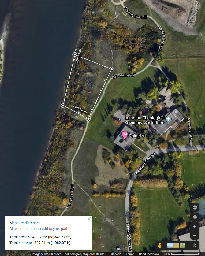
Study site updates: Due to the difficulty in navigating some of the steep slopes within my initial study area, and avoiding some areas that may confound the project, I have redefined my study site. The original study site was an area of approximately 38 576 m2 in size and encompassed a ravine. I desired to study the forb species abundance and distribution along the riparian-upland gradient on the eastern bank of the South Saskatchewan River. However, the ravine threatened to confound my project (having a separate species profile and elevation gradient), and some of the cliffs within the original study area were going to be too difficult to navigate. Therefore, the study area was reduced to 6 349 m2 and is depicted in Figure 1.
Hypothesis updates: My original hypothesis involved investigating forb species abundance and distribution as they relate to the distance from the river. However, I have now opted to shift my focus towards elevation (rather than distance). Furthermore, in an attempt to address the processes behind forb abundance and distribution, I have decided to estimate soil moisture along the gradient.
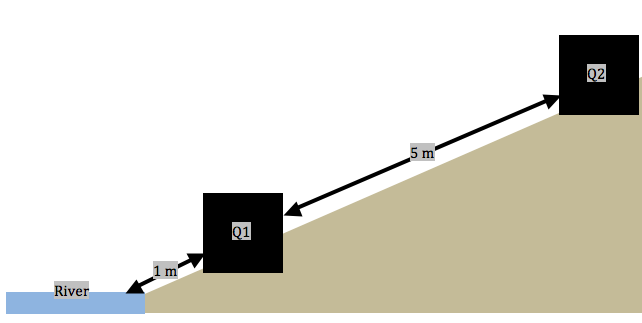
Sampling method updates: Following some advice and reflection on my proposed sampling methods, I have decided to adopt a systematic sampling approach (along transects) within the study area. Each transect will run perpendicular to the shore of the river and contain 11, 1 m2 quadrats that are spaced 5 meters apart (Figure 2). Ten randomly generated locations at the shore of the river were chosen and the first quadrat in each transect is to be laid at 1 meter from the river’s shore. Along these transects: I have been collecting forb species abundance, noting the proximity to river, estimating soil moisture (by hand texturing), and noting whether there is a tree/shrub canopy hanging over the quadrats.
Data Collection: Three replicates (transects) were sampled on August 5, 2020 between 9:30 AM and 6:30 PM. As stated above, each transect consisted of 11 sub-samples (quadrats).
Transects proved difficult to implement because the slope was extremely steep in some locations. Working from the river, I would lay a quadrat, collect data, then measure 5 meters to the next quadrat location. Some locations arose where I would not be able to move in a straight line (often up a cliff); therefore, I would have to mark the location of the previous quadrat, navigate to the new location via an alternate route, and measure backwards to maintain a consistent distance between quadrats. In addition, the upper area of the riparian zone is dominated by dense stands of Caragana sp. and Amelanchier alnifolia (Saskatoon berry) shrubs. This region was particularly time consuming to navigate; however, it was still feasible. The locations with a dense shrub canopy exhibited a notable absence of forbs. Therefore, at the sixth quadrat in transect one, I decided to begin noting when a canopy of shrubs or trees hangs over each quadrat. In order to maintain consistency, I navigated back to the previous five quadrats to collect this data before continuing to the seventh quadrat in the first transect. Overall, the largest problem in implementing my sampling technique was time. Not being able to complete all ten of my replicates in one day will mean that I may not have consistency with soil moisture between sampling days. This can be mitigated by ensuring that my sampling is, in the very least, completed within a timely manner (over the next few days). In addition, I will be navigating to some of my previous points on subsequent sampling days to verify that the moisture content of the soil has not changed. If it has, I will need disregard my previous soil moisture data and plan for an individual day of soil sampling to control for moisture variances.
Despite having only sampled from three transects, I am noticing ancillary patterns related to my hypothesis. The transects closest to the river are all saturated with water and this saturation level quickly declines as you move up in elevation. Consequently, many forb species exhibit preferences for different elevations. For example, Astragalus pectinatus (narrow-leafed milk-vetch), Cirsium arvense (Canada thistle), and Liatris punctata (dotted blazing star) display an extreme preference for dry (0-25% saturation), upland locations. In addition, Hedysarium alpinium (alpine hedysarium) and Astragalus americanus (American milk-vetch) are strongly associated with heavily saturated (75-100% saturation), low elevations. However, some forb species like Solidago canadensis (Canada goldenrod) do not appear to display a preference for any elevation or moisture content.
REFERENCE LIST:
Google Maps [Internet]. c2020. Canada: Google Maps; [accessed 2020 July 29]. https://www.google.ca/maps/@52.1378074,-106.6412387,549m/data=!3m1!1e3