Post 6: Data Collection

On August 3rd and 4th i collected the data from the remaining three of my four 10 x 10m sample plots, located along the shoreline of Nita Lake. Each sample plot was a replicate. Starting with Plot 1, i put into practice my now slightly more refined technique for determining elevation, with the series of 1 meter vertical poles and string running horizontally until it meets the slope of the shoreline. In the sub-1 meter elevation zone,  Alnus rubra grew densely and i had trouble counting the individuals without accidentally backtracking and double counting. However, i started flagging each tree as i counted them and walking up and back parallel with the shoreline boundary of the plot, recording the trees as i gradually made my way up the slope until i hit the back line of the plot. This made it much easier to ensure that i had an accurate tree count, without double counting or missing any individuals.

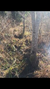
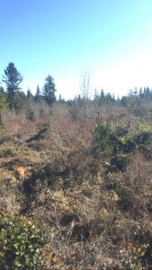
I have noticed that the substrate types in the sub 1 meter elevation zone are uniform across the four plots, which i believe could be a result of frequent flooding and erosion, creating deep, soft and moist soil substrates in the low lying areas. This could potentially compromise the testing of my hypothesis, as Alnus rubra dominance in low lying areas may be influenced by substrate type rather than correlating only with frequency of flood disturbance. However, for this reason i recorded all changes in substrate types throughout the different elevations, so by analyzing the species composition in different substrate types throughout  sample plots i should be distinguish and nullify the influence of substrate type in the flood prone zones.

Blog Post 6: Data Collection

I have completed my data collection. In total, I chose 15- 1 m squared replicates within each of my 16 transect lines. I intend to capture the spatial coverage of Himalayan Blackberry (Rubus armeniacus) in differing ecotone environments around my neighbourhood. I did this by measuring height and density (cover class).

My data collection went well, although it was hard to access some of my transect locations due to the bushes being un-passable. I had long pants on and big boots, then I paced one large step for every meter and would record relevant information. Areas where I could not access I would estimate height and location within the transect. I was hoping that by doing 15 – 1 m squared quadrats being slightly wrong on exact location would not influence my results too greatly, as I would still capture the general variability. I also did this in one day so growing patterns would not influence my results

I am starting to realize that Himalayan blackberry is opportunistic. I believe I am going to be able to disprove my hypothesis. Instead of preferring ecotone environments, the Himalayan Blackberry seems to be opportunistic appearing in most transitional locations.

Blog Post 6: Data Collection

I have had an interesting time collecting data in comparison to how I collected it in the field back earlier in the year. Collecting data using iNaturalist has been somewhat faster, however it does take time how to use it effectively and collect the data that I want. I have been able to collect 87 unique data points of bryophyte sightings located in various locations and elevations at the park. It has been difficult implementing my original sampling design since I am not able to physically collect my own data, so I have to work with what has already been collected. I have noticed patterns in species composition between the upper and lower portions of the park, but this will require further investigation as I begin to organize and analyze data. I plan to choose three to four bryophytes to perform the analysis on, due to the diversity of sightings recorded on iNaturalist.

Blog Post 6: Data Collection

Today I began my data collection activities for my project at along D’Herbomez Creek in Heritage Park. I’ve sampled 6 out of 10 transects, each with 10-15 quadrants. In this I’ve come across  a few challenges. For one, I say 10-15 quadrants because while I intended to sample 15 quadrants per transect, some steep slopes have prevented this from occurring based on my sampling model. I’m continuing with 15 where possible but the final analysis may be of 10 to eliminate the incomplete samples from the data set. I’m finding so far that 10 should be enough to disprove my hypothesis regardless. Another challenge I didn’t foresee and perhaps should have, is the thickness of the brush in places. My initial observations saw lots of good sampling areas, but my method of randomization has sent me straight through some thickets of blackberry and other shrubs. I’ve managed but it’s definitely not the same as sampling an open field.  As far as my hypothesis, it seems to have already been disproven based on the patterns (or lack of) that I am seeing thus far. The patterns I initially observed visually, and to a lesser degree experimentally in a previous activity, don’t seem to be holding up when other, randomly chosen sites are selected. This is somewhat disappointing, but even a false hypothesis adds to our understanding.

Blog Post -6

I started collected my data in month of April, during clear and sunny afternoon days. It was a very warm and windy day here in Vancouver Island. I just sat in observable distance from the feeder and spent an hour to collect the data. In order to thoroughly collect data, I decided to double the number of samples i.e. total 10 samples (days) in my final data and made replicates by including another feeder at my friend’s backyard in order to get supportive data for my hypothesis.  Before starting my sampling, I put the feeder for one day in order to let know the birds about it which I believe this simple adjustment helped me maintain a greater quality of samples and helped me record more bird species. I did not observe any new patterns during this exercise though I observed a unknown specie of bird so I named it as “unknown specie A”. The data collected seems to support my hypothesis.

Blog Post 6 – Data Collection

Data was collection was completed at Coquitlam River Trail, Friday, June 5th on a partly cloudy day. The temperature was 17 degrees Celcius. There is an abundance of growth in this area, which allowed me to be able to note which areas of the forest are shaded, and which are open to sunlight. The river is flowing steadily, and visible disturbance was present along the river’s edge, potentially due to overflow from snowmelt.

To get the most out of this project, I decided to double the length of my transects to 200 meters long. My original plan was to have 3 transects parallel to the river which were 100 meters long but found that there may not have been enough data if my transects were this short.

I sampled 3 replicates (3 transects parallel to the river) and used systematic sampling by area for my design. 10 quadrats were placed along each transect line, and data for Alnus rubra were collected, including the number present, and circumference of each. Soil moisture was tested in the center of each 10×10 meter quadrat with a soil moisture meter. Other trees within each quadrat were noted and circumference measured to assess for potential competitive interactions.

One issue I found with testing soil moisture, was that I was not always able to test the center of each plot due to gravel or rock. Therefore I tested the nearest patch of soil that was soft and able to read moisture. Now that the leaves are present on all plants, the identification of species has been much easier as opposed to winter.

My data collection supports my hypothesis that red alder require higher soil moisture. The quadrats with the highest soil moisture reading subsequently had more alder present. A pattern I noticed during sampling is that red alder and black cottonwood are both more abundant closer to the river.  Red alder are the only trees that lean into the river, while the black cottonwood grow straight up. This leads me to believe that there may be competition between these two species since they were often found in the same quadrats. I would also like to learn more about the interactions between salmonberry and red alder, as they were found to be next to each other most of the time. Because of the difference in size of these two species, I don’t believe there is a competitive interaction here, but that they are able to co-exist. A factor may be that they both simply thrive in areas of higher soil moisture.


Julia Thompson


Blog Post 6: Data Collection

Thus far, I have been able to identify shorebirds (to measure shorebird diversity) at 5 sampling quadrats at each location along the human presence gradient (gradient comprises three different sampling locations) 6 times. Hence, I have collected 30 replicates for each location along the gradient. I haven’t had any problems implementing my sampling design so far, except for the fact that it requires a lot of planning in regard to timing in attempt to control for timing variations of shorebird diversity. Thus far, it seems like shorebird species richness, evenness and abundance decreases across the sampling gradient. However, I would still like to collect more replicates for each location along the gradient to see if this effect persists with more samples collected.

Blog Post 6

My field data collection activities have gone well. After initial difficulties wrapping my head around how to actually test my hypothesis, I came up with what I believe to be a feasible experimental design.

Over the course of three months, I surveyed five plots in my study area. I chose random days to collect data, based on snow fall. After a period of snowfall, I would survey all five plots as soon as it got light enough to see in the morning. I measured temperature upon arrival with a Kestrel pocket weather meter. A survey would consist of measuring snow depth at the plot, removing my snowshoes too make less of an impact in the plot, counting mule deer tracks on the established snowshoe trail present in plots #1-#4, measuring snow depth of the established trail, counting mule deer tracks in both primary and secondary trails, and measuring the snow depths of each trail encountered in a plot. Before leaving a plot, I would re walk the established trail wearing my snowshoes a few times to ensure it was re-compacted. I surveyed all five plots six times between January and April.

The hardest part was accurately counting mule deer tracks on the established trail, as I would often have to observe several 60cm long grids to accurately count the deer tracks. In the -20C weather, this was a bit tedious-feeling some mornings.

I tried to keep my design fairly simple, and once I had switched from transects to plots, I had no issues implementing my design. I did not notice a threshold depth at which deer completely ceased to use secondary trails, as per my hypothesis. I am, however, fairly confident that at some point snow depth would become too great for deer to travel select travelling outside of an established or primary trail. It is impossible to say though in my study, as snow depth never reached a depth at which secondary trail travel completely ceased.

Post 6- Data Collection

I collected all my data over the course of two days this past week. I made 5ha boundaries on three zones in my study area (80 year old second growth Douglas Fir plantation, Riparian zone, and 18 year old harvested early succession) and randomly generated 10 GPS points within each area. I had numbered them so that I would navigate to the nearest next point to alleviate the frustration I encountered having to walk the same area twice as I did during the test trial the day before. I had spent some time studying how to estimate percent cover of vegetation and I had bear bangers this time. I encountered patterns that reflected my hypotheses: the black tailed deer sign was most abundant in the forest and the elk sign was most abundant in the grassy wet riparian zone. It’s likely I have enough data to show some correlation with deer and shrub abundance, but it seems more likely that the deer are more abundant in the forest because there is more cover from salal shrubs for security reasons not for food reasons, whereas there is not as much sign in the open harvested area due to risk factors associated with predation and less browse (although I imagine nocturnally they are slightly more active in this area). Why the deer spend less time in the wet riparian zone is not clear to me yet, and may be something to do with niche and resource partitioning with the elk (though I’m uncertain the elk population is large enough for this to be a factor). The elk sign it seems was correlated with the presence of high cover of grasses in the riparian zone, but I also found sign in both other areas leading me to believe they also feed on shrubs as they traverse the landscape, but prefer to stick to areas when there are suitable grasses to feed on.

Blog Post 6. Data Collection

Last weekend I collected a second round of samples from a Beaver Lake trail. In total, I sampled 10 replicates on 15 March 2020. The only problems I have faced so far with implementing my sampling design is identifying to the lichen genus level in the field. I have resolved this by taking photos in the field for desktop confirmations as well as written presence/absence notes for each replicate. I have also started grouping lichen observations by structural categories reported in the literature (i.e., crustose, squamulose, fruticose etc.)

There are also several sampling problems I have resolved. At first I was having difficulties identifying individual trees species in the field. I am now identifying trees to the family level, which is much easier. There is also scientific rationale for identifying trees at the family level when studying lichen because trees within the same family possess very similar bark. Since tree bark is the substrate used by epiphytic lichen, grouping replicates at the tree family level is appropriate.

I have noticed an ancillary pattern that has made me reflect on my hypothesis. I have noticed replicates along the periphery of Beaver Lake that appear to have more fruticose lichen types, and those identified as Cladonia sp. appear to have developed podetia (i.e., the fruiting body of the lichen). By comparison, the replicates sampled from the surrounding area that are buffered forest on both sides of the trail appear to have less fruticose lichen types and less have visible podetia.