Blogpost 6: Data Collection

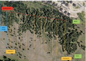
Collecting samples in the field has been fairly easy, so long as the proper amount of time has been allocated to collect them. In total, 450 replicates were taken using a 0.25m2 quadrat. These samples were taken randomly and in equal numbers throughout the three zone types as outlined in my experimental design; canopied forest, uncanopied forest, and open grassland. A total of 9 sampling regions were sampled, with 50 samples taken from each. Three of these regions were in open grassland, three were canopied forest, and three were uncanopied forest (Figure 1).


No major issues were encountered when implementing my sampling design (other than many mosquitos!).


So far, it appears that the grassland samples have a higher occurrence of Knapweed than in either of the forest zones; this would support my hypothesis that access to sunlight affects the growth frequency of Knapweed. Statistical analysis has yet to be done on the data.

Figure 1. Satellite view of natural area; uncanopied area not accurately represented due to
age of image (google maps). Rough sampling zones outlined; 50 random samples taken per sampled zone. Project total n= 450.


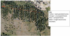
EDIT: A new data collection method was used following this blog post. 10 transects were sampled with 21 samples each, taken 10m apart along each transect (n=210). This new collection method cut the time needed to collect samples by a considerable margin. A 1m xx 0.5m quadrat was used to sample for presence/absence of Spotted Knapweed (Centaurea maculosa). See figure 2 for an updated design layout in the natural area to the South of residential Aberdeen, Kamloops.


Similarly, to the previous sampling method, grassland cover seems to have a higher frequency of Knapweed than either of the other two cover types. Data analysis still needs to be conducted to confirm the significance of this pattern.

Figure 2. ________. Natural area including walking trail south of residential area in Aberdeen, Kamloops. Coordinates for trail and trail head are 50° 38’ 1” N 120° 21’ 18” W. Elevation ranges from 860m at the bottom of transects (at trail level) to 935m at the top of transects. Transects are drawn in yellow, the walking path highlighted in red, and a blue length marker is included for reference; ten transects were sampled for presence or absence of Spotted Knapweed (Centaurea maculosa) and cover type (canopied forest, partially lit forest, open grassland) every 10m (total transect length 210m). Transect spacing was randomly chosen using a randomizer phone app. (total n=210).

Blog Post 6: Data Collection

I collected my data on August 2nd during the afternoon. It was a very warm and stormy day here in Florida. I managed to find a 2-3h window between two rainfalls to go collect my data on the field.

In order to thoroughly sample my site, I decided to double the number of samples or transects from my initial data collection in module 3. I then collected the same number of subsamples (or quadrats) per transects (10) but on 10 samples instead of 5. To do so, I had to collect my samples every 8 metres along the width of the field instead of every 16m.

Considering that I had collected my pre-experimental data from module 3 a few months ago, I decided to collect 10 new samples instead of only adding the 5 new ones to my already collected data. I feared that flower abundance might have changed with time and so I resampled everything.

The previous data collection that was made a few months ago greatly improved and facilitated my afternoon of August 2nd. The difficulties I had with keeping my transects straight were eliminated by the simple trick I elaborated months ago. Before starting my sampling, I would spot 2 or 3 checkpoints along the transect to keep it straight. I believe this simple adjustment helped me maintain a greater quality of samples.

I did not observe any new patterns during this exercise. The data collected seems fairly similar to the set collected months ago and so my observations and comments were the same.

Blog Post 6!

The field data that I have been collecting I was only able to have 5 duplicates because of the zone of the intertidal zone at McNeil Bay did not allow for anymore.The sampling design (transect with a randomly located sample plot) I chose works well because of the elevation in the study area. The quadrats were chosen systematically at random. I started with the top pool and always made sure the next pool was 2 steps away. The patterns that I have been able to notice are the richness in the low tide pools due to the better living environment (stays wet) and more cover there too. Another pattern would be the size of the tide pools depicting the species diversity since I’m only recording what is in the quadrat but there are many species outside of it.

Blog Post 6: Data Collection

Due to the size constraint of my backyard, I decided to modify the size of original and additional quadrats. I decided to decrease the size to 0.25min order to prevent the chance of overlap between replicates and to hopefully receive more accurate data in the process. In my initial data collection, I sampled at five locations using 1m2 quadrats. The three locations that I observed for my ongoing field observations are each unique from one another in terms of sun exposure throughout the day, the presence of dead grass and soil moisture. I then decided that the best way to select my first five replicates was to use the Stratified Random Sampling technique. I took one replicate from Location 1, another replicate from Location 2, and three replicates from Location 3. Using these replicates, I measured the percent cover of Common Fern Moss (Thuidium delicatulum) relative to a 1m2 quadrat size and used this data as a measure of abundance for this type of moss. Then, I calculated the mean percent cover of Common Fern Moss in these quadrats to get an idea of the area of my yard occupied by moss. I collected data on five additional replicates and had to recollect data from the original five plots using 0.25m2 quadrats. I had to resample the first five replicates because by decreasing quadrat size, the percent cover was expected to increase relative to the quadrat. This prediction was for the most part correct, as all values for the percent cover increased with decreasing quadrat size except for quadrat 5, where the value remained the same.

At this point, I have noticed a general trend in my data (with a few outliers) that supports my prediction and I have not yet reconsidered my hypothesis. I am seeing that areas in my yard that would typically receive more sunlight throughout the day have a smaller percent cover of fern moss in comparison with quadrats that receive more shade. My second data collection was in my mind successful, however, I hope that I can find a way to measure pH in these 10 and additional quadrats in order to factor in the impact of soil acidity on moss growth- I am sure I will find a way to go about that before my next data collection.

Post 6: Data Collection

On july 24th 2019 at 4:29 I began sampling more replicates for my  project. I have sampled an additional 10 sample units at this time. My sample design has been pretty straightforward and easy to replicate. The only problem I have run into is within the forested area some of the deciduous trees that have been observed are dying or recently died. I have decided to include these tree in my samples in a new category as deceased trees. If I observe significant dead trees within the closed canopy forested area I might be able to support my hypothesis with this data. So far my hypothesis “Does clear cutting, causing open canopies, have an increase in the amount of deciduous tree composition along the now exposed timber edge?” seems to be true. I have noticed a larger amount of deciduous trees along the cut block edge rather than within the standing timber

BLOG POST 6

I have started collecting data for my research project whose aim is to study the effect of soil and wind quality on the prevalence of the nodding onion plant in industrial areas surrounding my house. My area of sampling is divided into 15 sections. 5 sections located farthest from the industrial site, where the first to be sampled. The next 5 sections to be sampled was located at the equal-distance farthest and nearest industrial site while the last 5 sections to be sampled was located nearest to the industrial site. Each section consists of a quadrant. Therefore, in total, 15 quadrants were sampled for this project. The random sampling method was chosen to effectuate this study. Each quadrant was estimated to be 0.7×1.2m. At each quadrant, the nodding onion species was recorded and its cover was also measured. So far, I have measured 7 quadrants in this project. 2 quadrants farthest away from the industrial site, 3 quadrants nearest the site and 2 quadrants located at equal distance to the industrial site. I encountered several difficulties during the sampling procedures. Firstly, in some areas farthest from the industrial site, there was a significantly greater proportion of other plants most notably the Cow Parsnip (Heracleum maximum). Given the fact that this plant was taller than the nodding onion plant, it was sometimes difficult to locate this plant within a quadrant and record it.  Access to some sampling areas was difficult, therefore accurate results were not obtained for some of the quadrants. Due to the fact that I recorded higher than expected amounts of the nodding onion species in two out of the 3 quadrants nearest to the industrial measured so far, additional factors such as the amount of sunlight each site receives as well as the proximity of the site to surface water will have to be taken into consideration. At this point, I have not yet fully ascertained which variable has an effect on nodding onion abundance: Soil quality, wind direction, proximity to surface water or sunlight.  My hypothesis is centered on the effect of soil quality and wind direction. However, these other variables listed above will also have to be considered.

Blog Post 6: Data Collection

Blog Post 6: Data Collection

I have collected data on 10 additional replicates, five at Location 2 and five at Location 3 from my initial field observations. This brings the total number of replicates to 15. Replicate quadrat locations were still chosen using a simple random scheme. I modified quadrat size to 4m2 for quadrats near and around Location 2 (approx. 3 metres from the base of the slope) because the vegetation in that area included Saskatoon berry bushes (Amelanchier alnifolia) dominantly, a larger plant than the ferns sampled using 1m2 quadrats. In addition, at Location 3 (approx. 10 metres from the base of the slope) I modified quadrat size to 25m2 because I was beginning to sample fully grown trees. I would have liked to increase quadrat size to 100m2 but to accommodate 5 replicates within the physical constraints of the lot and slope size, I had to downsize. After quadrats were selected and sectioned off, I took measurements of area of species found within the quadrats, compared that to the total area of the quadrat, and converted this to a percentage of coverage. So far, my results and observations have not led me to reconsider my hypothesis. In fact, they support it. At higher elevations the species composition nearly entirely changes. Non-vascular common ferns (Athyrium filix-femina) were found to be dominant at location 1, whereas at location 3 the dominating species are highly vascularized and developed trees such as Lodgepole Pine (Pinus contorta) and Paper Birch (Betula papyrifera). This supports my hypothesis that the complexity of species found increases at higher elevations along the slope. A possible explanation for this is that plants at lower elevations are shaded from the sun by ornamental cedar hedges, standing at approximately 8 metres high, on the opposite side of the field.

Post 6

I have established 5 permanent sampling plots with 30 replicates (Western Red Cedar trees).  To date, I have had no difficulties in the field implementing my sampling strategy, but I did have to change my predictor variable from continuous to categorical.

I am beginning to think that my hypothesis is false, but it should correspond with another hypothesis.  My research has been monitoring the response of immature Western Red Cedar from the recent removal of the adjacent mature forest.  I predicted that the trees with the most sun exposure, as a result of logging, would die. Further research into the silvics of Western Red Cedar is helping to clarify my understanding of this organism. The reddening of the foliage after abrupt exposure to the sun is different than red flagging from drought conditions.

Frequently at work (as a harvest monitor) I observe that the equipment operators will retain a few understory trees as a “best practice” for clear-cut silviculture systems; However, usually, the Cedar trees die within the first few years of being exposed to full sun.

My question was:

Why wouldn’t the understory Cedar trees begin to thrive?  The trees have more available light, moisture, and nutrients after harvesting.

My other question which formed the focus for my research is:

What will happen to the immature trees when industry harvests next to an established plantation?  Harvesting can occur next to plantations as early as 7 – 10 years after the plantation has been planted.  Will the Cedar trees established along the boundary of mature forests be able to withstand the abrupt change?

Currently, it seems that I have underestimated the resistance of the immature Cedar.  Western redcedar is considered a stress tolerator with the ability to grow over a wide range of conditions (Antos et al, 2016).  It is the beginning of July and only a few trees are showing more than 1% of their foliage to be scalded from sun exposure.

Reference:

Joseph A. Antos, Cosmin N. Filipescu, Roderick W. Negrave (2016).  Ecology of western redcedar (Thuja plicata): Implications for management of a high-value multiple-use resource.  Forest Ecology and Management, Volume 375, Pages 211-222.

Blog post #6 – Data Collection

So far I’ve collected behavior data on 18 birds, with a goal of 150 (50 in the morning period, 50 midday, and 50 in the evening).  I’ve run into a few problems along the way and have made small adjustments to my sampling design as a result.

  • Initially, my study was going to focus on Mallard ducks only. I’ve noticed however, that at times I cannot find a single mallard on the pond.  The Mallard is just one of several species of “dabbling duck” present in the pond so I’ve expanded my data collection to all dabbling duck species. Thus far I’ve found Blue Winged Teal and Gadwall, in addition to Mallards.
  • It’s June in Alberta – Nothing makes you remember how quickly the weather can change for the worse around here than sitting on the far side of a pond without shelter!  I’ve had 2 data collection periods cut short by sudden bad weather so I’ve started taking advantage of “good” collection periods (ie: good weather AND a good number of ducks on the pond) by taking extra readings when the opportunity arises.  I still plan to collect the same number of replicates (150), will still keep my time frame to the same 3 hour windows previously stated, and will still strive to collect data on unique individuals at each visit,  however I won’t be strictly sticking to the “10 day: 3 collection periods: 5 birds per period” structure I’d previously designed.

I’ve noticed some interesting patterns in my observations.

  • The ducks I observe are frequently in pairs, usually a male and female, but occasionally 2 females.
  • In the evening collection period, I’ve been having a hard time finding ANY mallards to observe. I wonder if they live elsewhere and have returned “home” for the night?
  • The PM observation period is associated with a lower number of all birds, including species that I am not studying.

I don’t have enough data yet to draw any comparisons to my hypothesis yet, but I look forward to seeing if my ducks exhibit similar behavior patterns to ducks in natural wetland habitats.

Blue Winged Teal
Gadwall
Mallard

Blog Post 6: Data Collection

I have collected ten replicates, and it is going well so far. We had some hail storms on the weekend so it gave me variable weather which is what my project is on. My parameters were raining/not raining so I have added  an “other” column just in case there is any other atypical weather patterns for this time of year. I think I will probably do another five replicates to give a total N of 15.