Blog Post 5: Design Reflections.

My initial data collection based on my strategy went well. Since day 1 the density of geese around the waterbodies was obvious and the areas that I chose to collect data from were fairly close to each other. As I was collecting data I noticed that the number of geese around the ponds were much higher than around the river, which was supporting my initial hypothesis. The difficulty in my sampling strategy was regarding replication, I was not sure how to do that. So, I decided to count the number of geese at the 6 locations I chose twice a day and to also record the weather to see if that affected the number of geese. I counted counted the geese 5m around the ponds and river spots because they were in groups.

I was surprised with the data because there were so many geese around the ponds which I did not expect. I collected data using this strategy for 15 days. I also thought about dividing the grassland around just one pond into 10 quadrats and count the number of geese in them but I was not sure if that would prove my hypothesis, since I wanted to compare the density around 2 kinds of waterbodies. I achieved replication by collecting data twice a day in 6 spots so I did not modify the strategy. I decided to go ahead with my initial strategy because I wanted variation and more data to prove my hypothesis.
Blog Post 5 – Design Reflections

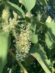
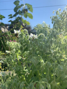
     So far I have not had much difficulty in actually implementing my sampling strategy, but I did have some questions to answer before initiating my strategy. Firstly, I had to consider that although I am observing honeybee activity in relation to the road, I had to find plants in each location that would be similar enough to sample the activity of the honeybees. I have chosen 3 plants that all contain flowers and leaves and seem to have honeybee activity regularly.

     After doing my replications, I was somewhat surprised with the results! At a quick glance, the elderflower shrub has an extensive amount of insect activity. But after observing the plant for 5 minute increments, I noticed that majority of these insects were not the Western Honeybee. Regardless of this, I was able to obtain some number for each replicate to add to my study.

     I think I will continue to collect data using the same technique as it makes the most sense for my study. I will keep the same plants I initially observed as I think they are the most similar and will assist in the accuracy of my study. Not only are these plants similar in looks, but they are also all cultivated plants which will help to keep my samples similar as opposed to having some cultivated plants and some naturally occurring plants.


Below is my replicate chart and the plants I intend on using for my study:


Replicate Number

Time of Point Count

Number of Western Honeybee Visits

1st

1259hr

17

2nd

1304hr

11

3rd

1309hr

9

4th

1314hr

14

5th

1319hr

15

Blog post #5: Design Reflections

My initial sampling day went as planned insofar as I was able to collect data using the method of walking a transect and placing my quadrat after a random number of paces. I was even able to find my target species in some of the quadrats and record useful data. My sampling plan was flawed, however, as it assumed a higher density of dog strangling vine. I ended up covering the whole length of my study area before I was able to obtain 5 quadrats containing the target species. The issue is that, while abundant, the vine grows in a small number of patches. My initial design attempted to avoid sampling more than once from each patch by having a minimum number of paces, but this turned out to be a problem as there are only 4 patches in the particular treatment area I was sampling. Further investigation revealed the same issue in the other treatment areas. My study area doesn’t have enough Dog Strangling vine patches to be sampled in this way.

The response variable data collected was generally as expected. The number of seed pods on the plants reflected the different treatment areas as predicted in my hypothesis. The soil moisture or predictor variable measurements were not as expected. All of the soil was measured to be dry, regardless of the treatment area. During the sampling it became apparent that this was another flaw in the study design. To demonstrate that the slope or manicured areas had less water than the area along the creek (which seems to be the case based on the compaction and visual dryness of the soil), I would need data throughout the growing season that showed the plants consistently had less water. A simple snapshot would not demonstrate this effectively.

I am going to modify my sampling approach in two ways.

First, since my sample unit is the individual plant, I am going to sample the various patches in greater depth instead of using random paces and quadrats along a transect. This will provide several replicate areas within each treatment and allow for a larger number of individuals to be counted. A quadrat will be used within each patch to collect 3 or 4 separate samples, several meters apart from each other. A random number generator will be used to determine random locations within each patch for sampling.

Second, since I can’t demonstrate that water availability is different across time between the different treatment areas. I will have to rethink my hypothesis. The data supports the observation that there is a gradient in the number of seeds between the different treatment areas so the predictor variable will be modified to be the different treatment areas themselves within the study area.

These two modifications will allow for significantly more individuals to be sampled within the study area while maintaining random selection, and allow for a hypothesis that is verifiable or refutable.


Blog Post 5: Design Reflections

My initial data collection day went as planned with implementation of my sampling strategy going quite smoothly. I came across one minor difficulty in that my home-made quadrat from cardboard, although useful, started to lose durability towards the end of the sampling intake due to the ground being moist/wet. As I took 10 samples in total, and my research project requires 20 samples in total, I will need to re-make the quadrat with cardboard and wrap it in plastic, or use a more durable material.

The data results were in support of my initial hypothesis prediction, however, I was surprising in that most quadrats did not have any presence of scat for both areas. I plan on collecting data using the same technique as it was quick, easy, good randomization, and allowed for easy visualization of any scat that was present in the quadrat.

Blog Post 5: Design Reflections

When I went into the field to start implementing my field strategy, I didn’t feel as if I had any major difficulties as I had prepared well before going into the field and had the appropriate tools needed. I think where the difficulties have now arisen is in my confusion of understanding the process. I chose to use a distance-based method (as this is used for stationary organisms, such as trees) and to use the simple nearest individual method as mentioned in Module 3 Sampling Techniques Tutorial.

I then used the Vegetation Resources Inventory (VRI) Ground Sampling Procedures from the Ministry of Forests and Range, which was extremely detailed and helpful, to supplement my understanding of the sampling strategy. I ended up implementing an integrated plot centre (IPC) quarter method which is what is now confusing me, as I am unsure if my sampling strategy is correct. My IPC was randomly chosen by splitting the area on the west side of Lost Lake into 16 zones then by using a randomized number generator to choose the zone. From here I used google maps to collect my coordinates to implement my sampling strategy.

I sampled 16 trees in total, four at the IPC and four at each auxiliary plot that are 50 metres north, south, east and west of the IPC. I was unable to sample at the eastern auxiliary plot as this was located in the middle of Lost Lake. At the IPC and the auxiliary points, I quartered the area using cardinal directions, into 4 sections. In each quarter I measured the DBH of the nearest individual (4.0 cm DBH) and measured the distance to the centre point.

Using the VRI ground sampling procedures it actually gets quite complicated for the quarter method as the data that I am trying to collect is tree attributes and the recommended sampling methods are fixed-radius or variable. When I dig further into this, variable plot is a method in which sampling area (plot size) varies with tree diameter and fixed-area, is exactly that, and you need to determine which trees are in or out based a fixed-radius.

To modify my approach, I may need to increase my sample size or alter my methodology. Either way, I plan to use tree attribute cards that have been provided in the VRI ground sampling procedures to help collect data clearly. I also need to document my access point, tie point and reference point. As I am in a municipal park I am unable to leave permanent objects or markings in the forest. Instead, I will look for obvious landmarks or unique trees that can act as these points. I also need to assess if I should replace my dropped auxiliary point, but this also answers if I should increase my sample size. All of these discussed modifications will improve my research to be standardized, repeatable and with little bias as possible.

Blog Post 5: Design Reflections

My initial data collection day went as planned and I was able to implement my sampling strategy with relative ease, despite plots landing in black hawthorn bushes and one plot that was inches away from a large hornets nest! I brought along an assistant (my wife) to help with note taking and tape measure holding which aided in the process.

The soil texture results were as I thought they would be with courses texture results on the steep slope section, with the exception of one plot out of a total of 20. Given my successful experience implementing my initial data collection I intend to continue subsequent data collection in the same way.

A possible modification I may make is the spacing of my plots and transect lines. Currently transect lines are spaced 10m apart with plots every 15m on each transect line. I insured that I evenly captured both the gentle and steep slope sections, however, I wonder if I should attempt to cover a larger total area. I could do this either by allocated more distance between transect lines and/or between plots.

Blog Post 5: Design Reflections

I conducted an area-based haphazard sampling experiment. I was sampling species diversity and vegetation cover in the garden. I didn’t have trouble with implementing my sampling strategy and i feel that I chose the most efficient strategy for the area I studied. I was surprised to see the abundance of fowler’s toads (Anaxyrus fowleri), this is most likely due to breeding season being late March- early June with the tadpole stage taking 50-65 days (Ontario Nature) meaning that there are many young toads living on land now. This could also be a factor to why there is an abundance of garter snakes (Thamnophis sirtalis) in the area since they are predators of toads. Another factor explaining the high toad density in the garden is the high vegetation cover, this supplies toads with an environment with suitable protection from predators, such as birds or rodents, and also lots of food, such as insects. I think that I will adjust my strategy by sampling a larger area so I can get a more in depth understanding of species diversity in the area rather than vegetation cover.

Young Fowler’s Toad

Blog Post 5: Design reflections

I did have some difficulties implementing my strategy. Randomly sampling made it hard to select which plant to measure when they were not as abundant in some areas. As well, trying to get an accurate representation from one plant branch of the plant became very challenging. The data was surprising because the plant heights between the two transects looked very different but ended up being very similar.

I will continue collecting my data with the same sampling method (random) with some changes. My data will be continued to be collected at random but i will measure several branches of each plant to average the height for each sample.

Blog Post #5-Design Reflections

I have decided to do an abundance study of frogs and toads of PEI and their distance from active farming sites. We only have four frogs-some will say five, but the pickerel frog hasn’t been seen here since 2003, and one toad. The green frog (Rana clamitans), the wood frog (Rana sylvatica), the leopard frog (Rana pipiens), spring peepers (Pseudacris crucifer), and the American toad (Bufo americanus).

My hypothesis is that the species abundance increases as the distance from active farming increases.

I have chosen five sites at random, however, I had to make sure that they had the right environment to support the frogs and toads, so they are all fresh-water riparian sites. I chose those sites and will be measuring the distance to active farming sites through arcGIS. I had some water chemistry analyzed at each of the five sites, however, I only had the funds for one sample at each site, so, depending on their nitrate and phosphorous levels, I will maybe only use this data in my discussion, to hopefully support my hypotheses.

I will drive to each of the five sites during the breeding season at dusk and record their calls for five minutes with my iPhone, then analyze the recordings using their call to identify them and the Abundance Code for Frogs to determine how many are calling:

0 = no amphibians heard
1 = individuals can be counted (no overlapping calls) – estimate of 1-5 individuals calling at site
2 = calls of individuals are distinguishable, but some calls overlap – estimate of 6-10 individuals calling at
site
3 = full chorus, or continuous calls, where individuals cannot be distinguished – estimate of more than
10 individuals calling at the site.

Frogs only call during mating season, so I intend to do 20 site visits (4 nights, at 5 sites) during this time.


Post 5: Design reflections

My initial data collection went well despite the weather factors and wildlife encounters I had to deal with. After many weeks of continuous rain, I was able to go to the site and stake out my study area. I initially was thinking of doing 250m2 based on my google earth location, however, on one side of my study location, there was an active great horned owl’s nest with nestlings that I had to keep distance to minimize stress. On the opposite side perhaps 500m away, a red-tailed hawk pair was nesting and were showing aggressive behavior when in the field. So, I decided to change my study location and study parameters.

With a 100m2, this still allowed me to transect along various zones being tallgrass, cottonwood trees, rocks and floodplain. I removed the upland slope and wetland from my study because of my constraints with the fence-line and wildlife. I added an extra sample to my transect making it 6 quadrats of 0.9144m2  in order to reach the floodplain.

I picked my transect lines at random with a random number generator. My intervals were 15m and sampling at opposite sides to increase randomization. Rather than using the x,y method to go parallel with each zone, I used the x, y method to cross each zone (perpendicular) from the fence-line to the river. I made a mistake by starting my first sampling at 80, 15 instead of sampling at 80, 0. To rectify this issue for my next transect, my options are: create my table with 80, 15 being my starting point; sample the missing quadrat point next time I go back; or select new random numbers and start over.

This will depend if the vegetation has changed and what time of the day I will transect. To improve overall uniformity and reduce bias, I am considering starting over. This wont take much time because I have created waypoints on my GPS of my x,y axis.

Overall, the systematic approach with transects and quadrats was the best method to use to increase my odds of observing absence/presence of ants along the gradient (response variable).