Blog Post #8 – Tables and Graphs

I initially made a table noting down the percentage of leaf color change for each of the five sections for the three trees I’m observing. I realized that the table was going to very long and almost a bit unnecessary. I finished it anyways and found a different way I could represent the same information. I mafe a new table with the same dates I took the observations, keeping humidity levels and time of observations. The only difference I made was making an average percentage of color change instead of having five different percentages for each tree. Now my table is more compact and easier to read.

Next I made a graph showing the color change over time. Three colors, one for each tree. It took a while to figure out how I was going to graph this and a way to assess it. There may be some changes later, bit everything seems pretty clear now.

The outcome was similar to what I expected, but I did wonder why these trees changed color slower than all the other trees. Could it have something to do with being in a highly maintained park by the city or is it because they were bigger trees compared to the other and were more able to collect resources they needed? Maybe it could be another reason too.

Blog Post 4: Sampling Strategies

Hello!

For the Virtual Forest tutorial, I used “Area” rather than “distance” and performed systematic, random, and haphazard sampling. The sampling technique with the fastest estimate sampling time was systematic at 12 hours, 5 minutes. following not too far behind was random sampling at 12 hours and 46 minutes and haphazard at 12 hours and 30 minutes. The percent error for the density of the 2 most common and the rarest species are as follows:

most common: Eastern Hemlock. Haphazard: 31.24% Systematic: 25.03% Random: 16.15%

Sweet Birch: Haphazard: 17.02% systematic: 53.87% random: 32.60%

rarest: White Pine. Haphazard: 1.20% systematic: 48.81% random: 50.00%

Striped Pine. Haphazard: 42.86% Systematic: 4.57% random: 76.00%

The accuracy did not seem to change with species abundance as there is no consistent trend between the standard errors for the common species and the rare species. as well, one sampling strategy does not appear to be more accurate than the others.

Blog Post 9: Field Research Reflections

Blog Post 9: Field Research Reflections

November 11, 2019


Throughout the course I analyzed abundant plant species in my back yard in Christchurch NZ. I created and followed through with the hypothesis that Hydrocotyle heteromeria, an invasive water species, is in fact limited by the moisture content in the soil. The soil on the South side of the lawn where the Hydrocotlyle was found contained high levels of moisture in comparison to the Northern side. The idea that one side of the lawn had higher moisture levels than the other is what led me to construct my hypothesis. I did however change my field study design. I was planning to analyze one single plot over a gradient, but I needed a complex computer program to analyze a design that contained one categorical and one numerical variable. I decided to create two plots, one which had ‘wet’ soil and one which had ‘dry’ soil. This change allowed me to create two variables which were both categorical and could therefore be analyzed with a tabular method using a statistical Chi-test. Since I changed my design it allowed me to add the completed data to my research paper instead of writing in my results “what I could have done” to analyze the data. I was glad that I could completely follow through with the results to determine if the variables were independent of one another.

I did however find it difficult to get enough research articles for my annotation. There was not a lot of relevant literature on my specific Hydrocotyle species. I did find a book which said that all Hydrocotlye species can be grouped into the same category because their biology was all extremely similar.

This course has been very worthwhile. It has given me practical knowledge to create and design research papers and field studies. It has also taught me various aspects on reading research papers which pertains to all courses and how to scrutinize research paper results to determine if the findings are credible. This course has allowed me to appreciate the dedication it takes to create large scale research studies.

Blog Post #6 – Data Collection

For my initial data collection, I only looked at three trees, systematically sampled on the North side of the park, as a whole, but as my observations went on, I decided to look at each tree in five different sections from top to bottom. For each of these sections, I noted down that percentage of leave that haven’t changed color yet, and then once I have all five sections, I took the average percentage of the total leaves that haven’t changed color. Each observation was initially taken three days apart, but after some revision, I decided it would be best to take observations every one or two days as the humidity level and leaf color changes more that I anticipated. This way, I could potentially get more accurate results.

I didn’t have too much trouble implementing my design, but there definitely had to be some changes like taking observations for frequently and using a hygrometer to better measure the humidity level.

So far, my observations do support my hypothesis that when humidity level decreases, than the leaf color change increases. But there are some observations that don’t follow exactly.

Blog Post Three: Ongoing Observations by E. C. Bell


Blog Post Three: Ongoing Observations by E. C. Bell

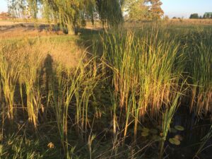
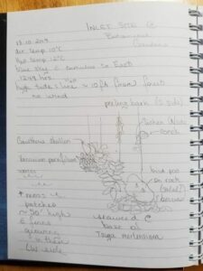
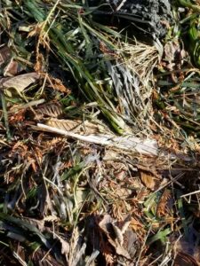
Feather embedded in seaweed, grasses & leaves at Inlet site.

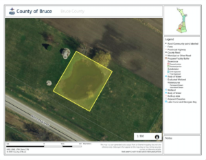
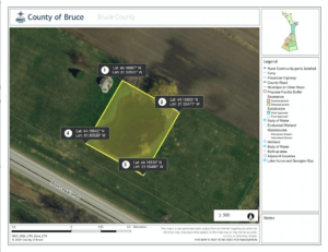
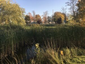
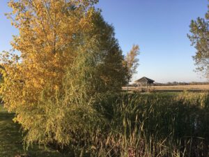
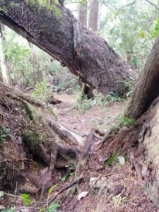
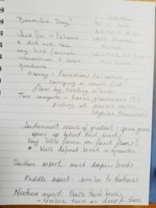
The biological attribute of interest of my study stems from the comparison of two gradients approximately 5km apart which have differences in physical traits of the transitions from forest to shoreline affected by environmental factors, including weather patterns and soil structure. The two gradients lie across Esowista Peninsula from each other, the Eastern inlet site and the Western coastal site. The ‘piece’ in this comparison will be the variance in ecotone transition and the ‘pattern’ will be the similarities in species with distinct differences in their physical traits and interactions. The elevation of the inlet location has a more gradual slope directly through the shifts in environmental factors. There are pebbles that increase in size to boulders of beach-ball size at the forest line, more of both seaweeds than grasses towards the pebbles, holding feathers, shells and bits of driftwood. The coastal site rises steeply for approximately 1m from sand to brush, covered in grasses, some seaweeds, yet then tapers off to a gradual slope covered in thick brush, mostly Gaultheria shallon. There is a fairly distinct line where stunted Pinus contorta takes over, looking very bonsai in shape of the needles with a sparse undergrowth – very little fauna of any species was growing on the forest floor. It was a messy situation getting through the thick brush.

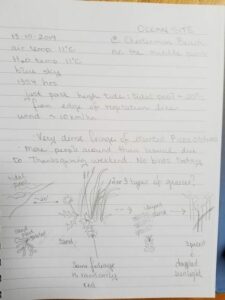
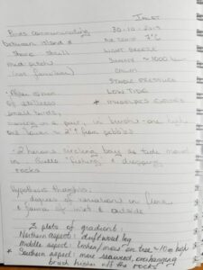
Western Coastal site                      Eastern Inlet site behind the shoreline brush

The hypothesis I am considering for this comparison of two environmental gradients is: there will be degrees of variation in the expression of populations and their densities within existing species due to tidal patterns and differences in weather exposure experienced over time. The ensuing prediction is: because of the different micro climates created by topographical land mass and Eastern facing aspect, the inlet site will have more biological diversity but less density in flora and interacting fauna than the Western facing aspect due to the open ocean exposure and pattern of winter storms, which have both shaped the gradients and variance that there exist. One categorical response variable may be variance in the dimensions of leaf size in Gaultheria shallon assuming that each location receives a similar exposure to sunlight. One continuous explanatory variable may be exposure to wind over a range of temperatures.


E. Carmen Bell

Blog Post 3: Ongoing Field Observations

The organism I plan on observing is English ivy (Hedera helix)

Since observing this vine-like plant last time I visited my study site, I researched the name of it and see that it is an invasive species in southwestern B.C.

When observing my study site, there is not a gradient of elevation, but there is a gradient of sunlight. There is a densely forested area that has lots of branch cover and little sunlight. Here the Ivy grows thick and covers stumps, fallen trees and the ground where the trail is not. Moving closer to the beginning of the trailhead, there is less branch cover and the ground is slightly drier. There are small patches of the Ivy, but the leaves are much smaller, and they grow in groups. Along the length of the open trail, there is no trail cover and the ground is much drier. Long grasses grow here, and there was no sign of the Ivy. It appears that sunlight is the underlying process for where the Ivy grows. Perhaps the plant is not so picky about where it grows/what species it is growing around but is more dependant on sunlight. This leads me to hypothesize that the English Ivy grows in shaded, damper areas.

The response variable here could potentially be the abundance of English Ivy growing (continuous) and the explanatory variable could be access to sunlight (categorical).


Blog Post #5 – Design Reflections

At first I wasn’t sure how I would measure the change in leaf colour with changes in humidity levels, but I think measuring the percentage of changed leaves this way is going okay. I couldn’t think of another efficient way of collecting this data. After four observations and noting down the humidity levels each day of observation, I may need to do more, perhaps every day or two, instead of three days like what I’m doing currently. This way, I may be able to see changes more steadily than a big change. I’m also going to bring out a humidity detector to more accurately measure the humidity in the park at that time.

I am surprised to see though, that leaves at the top of the tree changed much faster than those closer to the bottom. As well as seeing that leaves further on the outside of the branches change faster than the inner parts of the branches, where it is also more dense.

I’m not sure if I’ll keep how the data is shown in a table, but there is a way to better sum up all the information with a different visual.

Blog Post 6: Data Collection

During my initial observations I determined the size of my entire study area (Figure 1 and 2). The size of is approximately 28m by 30m, which I then divided into four quadrants 14m by 15m. As discussed in my previous post after trial and error it was determined individually counting the species to research diversity and population density of invasive pond weeds would be best represented in a range. By utilizing a chart, I have visited the pond a handful of times, once a week and made note of the population densities for various plant species, based on their location surrounding the pond (N,E,W,S) and the ratio of interacting factors.


Figure 1: Study Area


Figure 2: Study Area Coordinates

The following photos were taken October 20, 2019 at 5:00 pm on a sunny fall evening. The weather was approximately 10 degrees celsius and somewhat windy.

Blog Post 5: Design Reflections

Although my data collection may be more straightforward then other studies that involve in depth measurements and larger study areas, I still found I had some difficulty solidifying my study areas. Due to the fact the pond I am studying is irregularity shaped it was difficult to create study areas that were the exact same area and consistent with one another (i.e. similar amount of grassed area, pond water depth, etc). I used air photos and online mapping tools to create a rectangle surrounding the pond and then divided the rectangle evenly in four. The quadrants were divided by direction which was one pro as that is consistent, NW, NE, SE, SW and will be utilized as a variable. I found it difficult to conduct accurate population density of the species by counting for the heavily populated species since it was difficulty to differentiate between individuals and keep track, to counteract this I decided to create a range rather than an exact number. This may be subjective and difficult to confirm accuracy, so I repeated this population count once a week for 8 weeks. There was little to no variation between each visit, especially with mature vegetation like trees. However, I also believe this information is bias to the current season being fall compared to obviously Winter, Spring and Summer. I am confident supplementary research will assist me in supporting my data and I look forward to research pond management and diversity further.