The graph that I created from my collected data was easy to organize, aggregate and summarize. I had the data all laid out for each tidal zone (high, mid and low) therefore, I was able to group together zones and average data which would be more representative for a specific zone. The outcome was similar to what other papers have found but I still predicted that low-tide pools would have greater richness and diversity but this was not the case for all species. The mid-tide zone had more barnacles and also more snails which was not expected but this gave me the idea to look at other papers and they noticed this trend too. The mid-tide zone provides a good environment very similar to the low-tide zone. Making my graph has prompted me to look more into what environmental conditions the thatched barnacles prefer to live in.
Category: Nancy Elliot
Blog Post 7!
The theoretical basis behind my research is to study the diversity of species living in intertidal locations with varying environmental stress. It can also relate back to climate change with the sea levels rising will the species at high elevation still be able to survive. The ideas that are connected to my research include any study that is looking at elevation from the low-tide mark as a key factor in different species. Also, the idea that the ocean environment is changing and within these micro environments ( tide pools) they can show a small version of what could happen to the whole ocean with regards to less diversity with changing conditions (ie. sea temperature and sea level rising).
Species diversity, intertidal zones, marine niches.
Post 8
I would have preferred to display my data in a graph but because there was weak evidence for my hypothesis I felt it would be easier to interpret my data using a table.
I did struggle to collect the correct data for my hypothesis. After starting the literature review I was able to better understand why some western redcedar trees sunscald after they had been exposed to full sun, but others are able to thrive in full sun. Western redcedar is not shade requiring but rather shade tolerant, meaning they have adapted to both full sun and shade conditions. If I had understood the evolutionary fitness process of being able to develop two morphologically and physiologically different leaves (Shade leaves and Sun leaves) I would have set up my plots to study different replicates.
However, the slight increase in light conditions has shown some damage to the foliage on the trees that were adapted to sun exposure which will correspond to my hypothesis.
I would like to further research the ability for shade leaves to recover or adapt to sun exposure. To date, I have not been able to find any literature specifically related to western redcedar’s ability to recover from sunscalding. Or does the tree just shed the damaged shade leaves and it’s new growth develop as sun leaves?
Blog Post 6!
The field data that I have been collecting I was only able to have 5 duplicates because of the zone of the intertidal zone at McNeil Bay did not allow for anymore.The sampling design (transect with a randomly located sample plot) I chose works well because of the elevation in the study area. The quadrats were chosen systematically at random. I started with the top pool and always made sure the next pool was 2 steps away. The patterns that I have been able to notice are the richness in the low tide pools due to the better living environment (stays wet) and more cover there too. Another pattern would be the size of the tide pools depicting the species diversity since I’m only recording what is in the quadrat but there are many species outside of it.
Blog Post 5!
The collection of data in Module 3 went very well. A difficulty that I encountered was finding tide pools at the high tide region since most of them at McNeil Bay are at sea level. There were many more at the low tide region but I was only able to randomly select 5 from down below and had them spaced apart by at least 1 meter (2 steps). The water in the tide pools further down was quiet murky so it was hard to see what was inside all of the pools. Since I was measuring cover for the algae, I collected that data first and then looked for the individual species that could have been hiding underneath. The data that I collected was not overly surprising because I did see more biotic species (fish) in the pools closer to the ocean. I did however notice more seaweed cover at lower levels which I thought I would find more of higher up. I will collect the data in the same way for my final collection because I did not encounter any serious difficulties. I could improve the data collection by being more precise with the the sampling technique using transects along a measuring tape. This will improve the accuracy of pools that are in different elevation gradients.
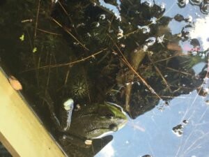
Blog Post 3: Ongoing Field Observations
The organism that I plan to study is the bullfrog (Lithobates catesbeianus) present at the Champlain Lake south wetland/swamp site chosen for observation. I had taken note that the stationary presence of a Lithobates catesbeianus in stagnant water appeared to be dependent on its location featuring sub-merged aquatic vegetation. None of the seven total observed Lithobates catesbeianus were present in an area of water that had no aquatic vegetation beneath the organism.
The three locations I have chosen to observe the organism of interest is the interior small channel flowing south, the main open body, and the lake mouth channel running into the wetland body (see photo for location references).
- Location 1: Interior small channel (south flowing)
The water in the wetland had dropped approximately 1 foot, leaving the channel to be very shallow and featured minimal room for aquatic vegetation. The channel was very stagnant and I did not observe any bullfrogs (Lithobates catebeianus) present in this area. I assume their absence in this channel was due to low water levels causing restriction for travel along the channel. - Location 2: Main Open Body
The main open body of the wetland also had signs of lower water levels along the shoreline, exposing previously submerged rocks and some dried up aquatic vegetation. This location had the majority of Lithobates catebeianus present and featured ample aquatic vegetation beneath each organism. I noted in my field journal the surrounding areas lacking visible aquatic vegetation, also lacked the presence of a Lithobates catebeianus. The water was very stagnant in this location as well. - Location 3: Lake Mouth Channel (running southbound into wetland body)
The lake mouth channel had a few sections of submerged aquatic vegetation and featured one smaller Lithobates catebeianus on the interior side of the channel. This channel had slight/low flow entering southbound into the wetland body and I predict the lack of Lithobates catebeianus presence throughout the lake mouth channel location is due to minimal aquatic vegetation coverage and difference in water velocity.
I postulate that the presence of a stationary Lithobates catebeianus is dependent on ample (>50%) coverage of submerged aquatic vegetation beneath the organism. Based on the postulate hypothesis, one potential response variable could be the Lithobates catesbeianus and one potential explanatory variable being the percentage of submerged aquatic vegetation coverage. The response variable would be categorical in this case, being the presence/absence of the Lithobates catesbeianus, and the predictor variable would be continuous, being the percentage of aquatic vegetation coverage. I expect the Lithobates catebeianus is stationary in water with ample aquatic vegetation beneath the organism to evade other predators present in the wetland.
I had a few images to accompany this post, however, are too large to include.

Blog Post 3!
I plan to study the tidal pools at McNeil Bay in Victoria BC. The organisms that live in these pools are both biotic and abiotic. Examples are barnacles, fish, brown and green algae. The abundance of these organisms varies depending on the zones of the pool from high tide to low tide. The three locations I chose to observe the changes in were low tide, intermediate tide and high tide. Below is some notes that I recorded on the locations:
- Low tide: Greater biodiversity, the organisms here do not need to be well adapted to drying out and extreme temperatures. Organisms such as anemones, brown seaweed crabs and fish live here.
- Intermediate tide: At this point there is a mixture of both species in the low and high tide but mostly it looks like there are a few invertebrates (chiton) but lots of seaweed.
- High tide: Organism here have to survive drying out, currents and wave action. A larger abundance of barnacles, seaweed with only a few invertebrates can be observed.
These patterns could be due to the very different environments that they live in varying with elevation. I hypothesize that low tide zones will have greater abundance than high tide for (species) due to the less harsh conditions for it to live in. I predict larger biotic organisms are only in low tidal zones. Based on my hypothesis one potential response variable would be the total number of each species in the tidal pools which is categorical. A continuous variable would be the percentage of cover of each pool with seaweed. One explanatory (predictor) variable would be the unique environment the tide pool provides for the species. This variable would be categorical since there are 3 distinct locations of the pools.
I am not very good at drawing so I only sketched a few things but mostly I have chosen to take pictures and document my field observations all electronically.


Blog Post 4!
This post describes the results from the virtual forest tutorial!
Result Summary- All Sampling Techniques (Here is a link to visually show my results).
The shortest estimated time to sample was 4 hours and 49 minutes for the distance, random or systematic.
Comparing percentage error between species for the most and least common species:
Red maple: (distance systematic, area haphazard, area random) 24.8%, 12.5%, 6.3%
White Oak: (distance systematic, area haphazard, area random) 50%, 4.9%, 51%
Yellow birch:(distance systematic, area haphazard, area random) 100%, 100%, 100%
White ash:(distance systematic, area haphazard, area random) 100%, 100%, 100%
Most accurate for the most abundant species: Area, random
Least abundant: American basswood was only picked up on the distance systematic. The accuracy decline with the rare species compared to the more dense species.
I propose that more than 24 sample points would have given a better overview of the area. There were rare species that were not sampled so with 40 points they might have been. 24 was enough sample points to measure the larger species but for the smaller ones more points should be used.
Post 7: Theoretical perspectives
My project is studying the effects of clearcutting on species composition along the newly harvested edge. Some ecological process my hypothesis touches on is the rate at which a forest re establishes itself and the successional stages it goes through. Another process that my project touches on is the effects of weather on a newly exposed edge of timber due to clearcutting. This part of the study will be interesting to determine how the now open canopy receives additional resources needed for growth but also is subject to new challenges. Three key words that pertain to my project are Open Canopy, early successional species and site disturbance.
Post 6: Data Collection
On july 24th 2019 at 4:29 I began sampling more replicates for my project. I have sampled an additional 10 sample units at this time. My sample design has been pretty straightforward and easy to replicate. The only problem I have run into is within the forested area some of the deciduous trees that have been observed are dying or recently died. I have decided to include these tree in my samples in a new category as deceased trees. If I observe significant dead trees within the closed canopy forested area I might be able to support my hypothesis with this data. So far my hypothesis “Does clear cutting, causing open canopies, have an increase in the amount of deciduous tree composition along the now exposed timber edge?” seems to be true. I have noticed a larger amount of deciduous trees along the cut block edge rather than within the standing timber