Blog Post 7


My project is around fern growth in relation to varying amounts of sunlight. I have broken the areas I am sampling in to either be shaded, partially shaded or no shade. My hypothesis is that ferns will be more abundant in shaded areas. This is something that I have observed while finding suitable sites for sampling. From my initial sampling the partially shaded areas have the most ferns. Likely there are several other variables influencing the growth of ferns. The amount of water, human disturbances, intraspecific competition, change in gradient which can influence water. The human disturbances occur from one of my sites which is cut every several month by the gas pipeline owners. In this one sites there are almost no ferns possible because they can’t compete with the faster growing prickle bushes and grasses. I plan on taking more samples to provide a more clear picture as to what lighting conditions are optimal.


Keywords: Fern abundance, light adaption, light gradient.

Blog post 9

There were several difficulties during the field research, especially when designing the field experiment and carrying it out.

First, in the step of designing field experiment I had difficulties in deciding response variable that represents what it was meant from hypothesis. The hypothesis is that overall ecology are healthier and varies in species as more artificial land development induced in the region. Independent variable was 3 levels of landscape that differs in land development. While response variable was hard to decide because it needed to represent the vegetation was healthier. At first I thought of measuring the ratio of green grass and dry grass would represent the health of vegetation, ecology. However, I didn’t put in the consideration that three landscapes had way more species other than grass. So, I decided to count the number of species that can be counted within in the quadrat also, I decided to count the green area per quadrat to represent the health of ecology. I also didn’t want to measure merely vegetations so I decided to measure bird activities as well. All three experiments later wards represented the intention of the experiment well.

Also, in the step of implementing the experiment I had issues in choosing sampling techniques. As the landscape were very small quadrat was easily overlapped when I was using random sampling techniques. This might lead the data to be inaccurate. Therefore, I decided to change the sampling technique to systematic. This helped getting more accurate data and observations.

Although my research project was limited in small region and there was not enough samples to support the hypothesis. I realized that practicing an research study, especially on ecology, would be way much more harder than I expected. It was hard to design an appropriate experiment that supports the theme and whether it represents well. Also in the process of carrying out getting the data from the field required a lots of commitment. Due to this project, I had a good time to appreciate of how ecological theory had developed.

Blog post 8

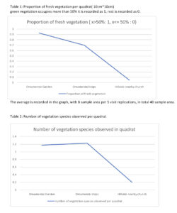
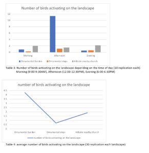
I have made 4 graphs in total to represent my observation for my research project. Graph 1 describes proportion of fresh vegetation per quadrat. The outcome turned out as I expected, the area that had least human management had the least healthy vegetation. While, the area that had most human management had the most healthy vegetation. Graph 2 describes the number of vegetation species found per quadrat. I assumed that there will be the most vegetation species on ornamental gardens and least on the preserved hill and the graph result showed somewhat different results. Ornamental steps had the most various vegetation species per quadrats compared to ornamental gardens yet preserved hill had the least various vegetation species growing in the landscape. Graph 3 describes the number of birds activating on the landscape depending on the time of day (10 replication each). This table demonstrated the bird activities depending on the landscape and time of the day. It was difficult for me to see overall trends of bird activity because the results were showing in so much detail in Graph 3. Therefore with the same data I made graph 4 to represent overall bird activity rate depending on landscape to observe easily. The activity of birds data revealed that did not expect when I started the experiment. I assumed that as ornamental garden had most healthiest vegetation, there would be the most bird activity among the landscape no matter what time in the day. However the results turned out that in the morning and evening the hillside church has the highest bird activities and the ornamental steps were the lowest all the time. This result lead me to a thought that bird activity might not be affected by healthiness of vegetation, instead it might depend on type of vegetations. Further exploration, I decided to study types of species generally found in all the landscapes.

Blog Post 7

The hypothesis that I set out is the overall ecology are healthy and varies in species as more land development induced in the region.


Land development involving human activities are sort of artificial selection activity. We measured the health of ecosystems in many ways by taking into account different sides  to measure their health. And the health of ecosystem depended on the landscape. Whether the landscape was actively managed by human was the independent variable, which derives in different environment where individuals shows different survival and reproduction rate. This offers an context with natural selection and artificial selection among ecological concepts.


Keywords that I would use to describe my hypothesis would include artificial selection, evolutionary fitness, vegetation abundance and diversity, bird activity, urbanization.

Blog post 6: Data collection

Create a blog post describing your field data collection activities. How many replicates did you sample? Have you had any problems implementing your sampling design? Have you noticed any ancillary patterns that make you reflect on your hypothesis?


I have implemented three data collection activities to recognize the healthiness of ecology depending on humans intervention rate.

First observation  was collecting the ratio of fresh vegetation per area. Fresh vegetation proportion was measured by the colour, green. In a quadrat (10cm*10cm), if the area is composed of greens more than 50%, it would be recorded as 1. If the area observed had green vegetation less than 50% of the area,  it was measured as 0. Each landscape, ornamental garden, ornamental steps, and preserved hill side, was measured 8 quadrats and it was measured with 5 replication. Since the area wasn’t that big, the quadrat selection might overlap easily. I had to use systematic sampling techniques. The area was divided into 5 area and quadrates were selected in subdivided area per visit. After one visit the other area was selected for data collection. In this way, overlapping of quadrat was avoided.

Second observation was collecting the number of vegetation species observed per quadrat (10cm*10cm). As above the area was divided in to five and subdivided area was observed each visit. 8 quadrats were observed per visit and was measured with 5 replication.

As going through both experiment 1 and 2, there should have been consideration of the amount of water the land received and type of soil the vegetation grows. They both affect highly in vegetation growth. The hill nearby the church isn’t actively managed by someone, the amount of water the landscape receives and type of soil they grow on might be different. On the next observation, observing this point is another important criteria.

The third observation was measuring the bird activity rate depending on landscape. Bird activity should be considered morning, afternoon and evening. The bird activity rate changes during the time of the day. Therefore, each visit per day must be three times; morning (9am-9:30am), afternoon and evening, with 10 replication. Each observation lasted 10 minutes and the number of birds flying around the landscape was measured.

Post 6

Background: I have decided to change my hypothesis and organism I am studying to make my sampling simpler. I have observed that deer fern are more present in some areas of Burnaby Mountain covered in forested than areas than areas that don’t have trees. To keep this simple I will categorize a sampling area as either shaded having most of the sky covered by the tree canopy, partially shaded having part of the sky shaded and non-shaded. These three zones represent differing levels of sunlight that is able to reach the ferns on the ground. My new hypothesis is that the deer ferns are more successful under lower lighting levels. As such my prediction is that I will find a greater abundance of ferns in shaded and partially shaded areas than non-shaded areas.

I chose three sites to conduct my sampling each had a non-shaded area, partially shaded area and shaded area. At each area I recorded 10 samples. For a total of 90 replicates. My sampling unit was 1m2. Which I had planned to measure the ground cover of the ferns; however, I found that most ferns covered the whole area. So instead of trying to measure ground cover I just recorded either the area being mostly covered by deer fern, grass, bare ground, tree or thorns. Of my three sites one of the non-shaded areas is managed to some extent because a gas line is below so they clear cut the area every few months. I think this has had the effect of reducing the amount of ferns that can grow because they are in competition with other plants that perform better under higher lighting conditions. The partially shaded zones had the most ferns with 15, shaded at 5 and no-shade at 6. This is what I had initially observed; however, I had expected to find more ferns in the shaded areas. I observed in the shaded areas underneath the trees (evergreens) that very little grew, the ground was mostly covered in pine needles. In the partially shaded areas the trees were mostly thin in diameter deciduous trees. One of the non-shaded areas had a high number of ferns which was the opposite of the other 2 non shaded areas that had only 1 fern each.


Blog Post 4: Sampling Strategies

Systematic sampling (area):

Sampling time= 12 hrs 7 min

Hemlock= 637.5….Percentage error= (35.67%)

Red Maple= 116.7…Percentage error= (1.85%)

White Pine= 8.3…Percentage error= (1.19%)

Striped Maple= 12.5…Percentage error= (28.57%)

I was surprised when I found that the most abundant species was represented so inaccurately while the least abundant was very accurate. I believe this may have occurred because the quadrats followed a very specific gradient going south to north, therefore we miss out on the other species that may be more present to the east or to the west of our selected quadrats.

Random sampling (area):

Sampling time= 12 hrs 42 mins

Hemlock= 420.8….Percentage error= (10.45%)

Red Maple= 100…Percentage error= (15.91%)

White Pine= 16.7…Percentage error= (98.81%)

Striped Maple= 20.8…Percentage error= (18.96%)

Overall this was even more inaccurate than the systematic sampling, especially with the rarest species- White Pine. By chance, the program sampled double the proportions of White Pine than are actually in the forest which is surprising. The more abundant species were more accurately represented.

Haphazard sampling (area):

Sampling time= 12 hrs 46 mins

Hemlock= 420.8….Percentage error= (10.45%)

Red Maple= 104.2…Percentage error= (12.4%)

White Pine= 0…Percentage error= (100%)

Striped Maple= 12.5…Percentage error= (28.60%)

This was the most inaccurate of the sampling techniques with not a single White Pine being sampled. This does not surprise me as their actual representation is quite low and haphazardly choosing quadrats without attention to the different gradients could easily lead to this result. The species in abundance were more accurately represented which is what I would expect.

Conclusion:

The systematic sampling technique had the fastest sampling time and was the most accurate. As long as the entire sampling area had similar environmental factors such as sunlight exposure, space, soil type/quality, etc then I feel this would be the best technique to use. If the environment was more diverse, more sampling points would be necessary in order to correctly represent the gradients. Either way, an increase in sample points would have been beneficial as I think would always be the case, but then that is more time consuming.

Blog post Four:

Community Sampling Exercise by Carmen Bell 

 Community: Snyder-Middleswarth Natural Area 


The three virtual sampling strategies used to assess species density for the Snyder-Middleswarth Natural Area included random, systematic and haphazard. Of the three, the area-based haphazard sampling method was the fastest at 12 hours, 12 minutes, likely because these are known representations of the larger area taken in a non-random manner. The longest duration was the area-based random or systematic method of 12 hours, 45 minutes. The difference in time between the two is not vast for the 24 plots, however, the difference may increase given more sample points.  


1. Area, random or systematic  2. Area, random or systematic  3. Area, haphazard 


12 hours, 35 minutes  12 hours, 45 minutes  12 hours, 12 minutes 


For the total area of the Snyder-Middleswarth Natural Area, 24 sample points were not enough to represent the diversity of the 200ha old-growth hemlock-yellow birch forest. In effect, each sample point represents 8.3 hectares (20.6 acres) over the steep terrain of a ravine created by the Swift Run River. As this is a virtual exercise, the representation can only be imagined. In a real case scenario, the accuracy represented in the sample points would depend, in part, on the variation of soil composition within the degrees of steepness. 


My assessment of the histograms from a perspective of relative species abundance, determined that the Eastern Hemlock and Sweet Birch be considered common, while the remaining species be considered rare. Within the context of biodiversity, “…, n individuals usually fit a hollow curve, such that most species are rare … and relatively few species are abundant” (McGill, et al., 2007). Each of the Yellow Birch, Chestnut Oak, Red Maple, Striped Maple and White Pine had a relatively hollow curve given the limited data. The Snyder-Middleswarth Natural Area is known as an old-growth hemlock-yellow birch forest. The lower density of yellow birch could be attributed to the larger stem size of an old growth tree. 

Considering the Eastern Hemlock and Sweet Birch as the most common species, the most accurate density reading was the Eastern Hemlock with a 10.6 percentage error between the known and sampled data. Considering the Yellow Birch, Chestnut Oak, Red Maple, Striped Maple and White Pine species as rare, the most accurate density reading lay with the Striped Maple at 14.3% error. I would like to point out that only 20 trees were sampled with a known density of 17.5. The Yellow Birch had a higher percentage of error at 30.2, however, the known density is 108.9 with 76.0 represented in sample data, demonstrating a stronger representation of the species.  


Eastern Hemlock

                 Actual   Data

Density  469.9  520.0 


520.0 – 469.9 / 469.9 x 100 = 10.6% percentage error 


Sweet Birch  

Actual   Data

Density  117.5  188.0 


188.0 – 117.5 / 117.5 x 100 = 60.0% percentage error 


Yellow Birch

Actual   Data

Density  108.9  76.0 


76.0 – 108.9 / 108.9 x 100 = 30.2% percentage error 


Chestnut Oak

Actual   Data

Density  87.5  36.0 


36.0 – 87.5 / 87.5 x 100 = 58.9% percentage error 


Red Maple  

Actual   Data

Density  118.9  152.0 


152.0 – 118.9 / 118.9 x 100 = 27.8% percentage error 


Striped Maple  

Actual   Data

Density  17.5  20.0 


20.0 – 17.5 / 17.5 x 100 = 14.3% percentage error 


White Pine

                 Actual   Data

Density  8.4  0.0 


0.0 – 8.4 / 8.4 x 100 = 100% percentage error 
 

Blog Post 3: Ongoing Field Observations

Organism being studied: Alnus rubra (Red alder)

Gradient: The tree line of a forested ravine, the level top of of a slope before the shoreline, the shoreline itself which consists of boulders, small trees, mixed shrubs and perennials.

Alnus rubra is much more dominant along the shoreline and potentially non-existent along the tree line. This could be due to sunlight, a preference for more well-drained and less rich soil, or maybe Alnus rubra has a tolerance to the salt exposure (from the ocean) and has been able to outcompete other less tolerant species. It may also be that because its the only small tree species along the shore it’s much easier to spot than looking into a thick tree line.

The trees almost seem to have formed a natural spacing between individuals as well with none closer than roughly 20 meters. These specimens all seem quite mature considering the harsh environments in which they grow (taller than 20 feet with stems more than 8” in diameter). Even though these trees are well-spaced and have an abundance of flowering and fruiting bodies, I could not observe any seedlings or juvenile specimens in any part of the gradient.

Hypothesis: The mature Alnus rubra in this region, despite an abundance of flowers and fruit, can no longer reproduce in this location via seed.

Formal prediction: The number of Alnus rubra seedlings and/or juvenile specimens recorded will be very low or non-existent along the shoreline and at the tree line. Due to a change in some environmental factor (or factors) mature specimens have survived but their seed cannot germinate or the seedlings cannot survive.

Potential response variable: Continuous. The number of immature Alnus rubra along the gradient.

Potential predictor variable #1: Continuous. The number of mature, seed-bearing Alnus rubra along the gradient.

Other potential predictor variables:

Categorical- Soil type along gradient (sandy, loam, clay, etc)

Continuous- pH and/or nutrient composition along gradient.

scan_p205726_2020-01-06-06-52-58

Post 5: Design Reflections

I found my sampling strategy difficult to implement in that the samples could be clumped close together. In order to eliminate this difficulty I could try adjusting the number of steps associated with the random number generated, for example, only taking 10+ steps from my starting points instead of 9 or less.

I also found the data gathered to be difficult to work with. Douglas Fir circumference and ambient temperature do not seem to provide much information on their own in such a short timeframe. In order to make this data easier to interpret over the duration of this study I would like to add quadrant aspect and the relative subject population within each quadrant.