Blog Post 1: Observations

Time: 8:30AM on Dec 30 2019

Weather: Cloudy

Size and Location: Cristopherson Steps in Surrey, BC. The natural areas alongside the stairs as well as the roughly 2 km stretch of beach front at it’s base.

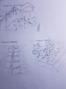
General description: The stairs begin from a suburban street and go steeply down a ravine, eventually over a railway track and to a beach. It’s quite rocky in this area and the shoreline is eroding from both the sea on one side and the regular removal of plants from the track area behind.

Designation: Cristopherson Steps is property of the City of Surrey but in the beach front area it is a mix of City of Surrey, BNSF Railway and potentially the provincial government because the tide comes very close to the area of interest.

Vegetation: Natural area alongside the stairs and down the ravine is mostly infested with ivy but there are also ferns, western red cedar, douglas firs. The beach front consists of deciduous shrubs and trees, and a mix of perennial and annual weeds.

3 intriguing questions:

  1. There are very young western red cedar trees no more than 6 feet in height that have germinated from seed presumably from the few larger specimens above (some are growing inside or along decaying tree stumps, therefore I don’t believe they have been planted). English ivy is already climbing these young trees and I wonder if western red cedar can survive without removing the ivy.
  1. Along the beachfront the shoreline in front of the railway tracks is built up with large boulders. The areas that have Rosa and Holodiscus discolor growing within the cracks of boulders seem to be less eroded than the areas without. Do these plants stabilize the area better than the other more eroded areas? 
  1. The heavily eroded portions of the shoreline are sparsely populated with what I believe is Digitalis. I could not find it present in any other areas except where the shoreline has recently collapsed and the soil conditions seem poor. Are the areas where the shoreline has recently collapsed from erosion providing this plant with the conditions it needs to germinate and then not be out-competed by other plant species?

Field notes 1

Blog Post 9: Field Research Reflections

For my research project, I measured the abundance of English ivy in high-light and low-light conditions. The high-light environment was uncovered by tree canopy and the low-light condition was covered. I found that the abundance of English ivy was significantly higher in low-light conditions. Throughout researching, I did not have to make any significant changes to my research design and data collection went relatively smoothly. After collecting the data and reading the current literature I found this to be a very interesting topic to research and learn more about. Although my study design was relatively simple, it fits nicely in the literature and addressed some gaps.

This was my first time taking an ecology course and I have a much deeper understanding and appreciation of how ecology theory is developed and tested. it was very interesting to gain first-hand experience developing a research question and creating an experiment to answer it.

Blog Post 5

Background: I completed five transects each five meters apart.  Each transect consisted of five 1m2 sampling areas alternating from left to right 1 meter apart. For a total of 25 sampled spots. My sampling unit was the presence of fomitopsis pinicula in a 1m2 area. I only found 4 of the fungi in my sampling area. They were all living on dead tree stumps.  I think the presence of the fungi is very dependent on the location in the forest because it mostly grows on dead stumps. From my observations certain areas of the forest have very few stumps compared to other areas.


Difficulties: There were several problems I ran into:

  1. I used a measuring tape to measure out the distances which was time consuming and inaccurate at measuring the 1m2
  2. My study area is on a mountain which is difficult to walk up and down making the process arduous.
  3. I did not find very many samples of the fungi which I know can lead to statistical errors because of the low number of samples.
  4. The 1m2 was used because this is the most common unit I saw. I think because the fungi are not like grasses or other plants that can grow everywhere on the ground coverage this may not be an efficient unit to measure.


Modifications: I plan on making the following modifications:

  • Increasing the transect size to cover more ground. I think increasing it from 5 meters to 10 or 20 meters. An increase in my unit from 1 m 2 may also help.
  • Using a pre measured string to measure the areas to have more accuracy in the measurement.


The modifications would hopefully help me find more of the fungi and have more accurate measurements.

Post 9: Field Research Reflections

Upon reflection of my study, there are many things that could have been changed in order to make the study more critical with less room for error. Most of these errors could have been avoided but the concept and repercussion of the error were not realized until it had been made. Implementing the design that was originally derived was simple enough but lead to problems when it became evident there were many possible predictor variables at play. This sample of the practice of ecology has led to a significantly greater understanding when it comes to the scientific process and ecological theory. The process of turning an idea into a testable hypothesis is now much clearer. It is also evident how important the scientific process is in regards to ecology. Without the scientific process ideas around ecology would remain ideas and never make it to scientifically proven fact.


Blog Post 4


Technique: Systematic Sampling of Area

Sampling Time: 12 hours 7 minutes

1 Most Common Species: Eastern Hemlock

Actual Density: 469.9

Data Density: 425.0

Percent Error: 9.5%

2 Most Common Species: Sweet Birch

Actual Density: 117.5

Data Density: 95.8

Percent Error:    18.4 %


1 Rarest Species: white pine

Actual Density:  8.4

Data Density:  0.0

Percent Error: 100 %

2 Rarest Species: Striped Maple

Actual Density:  17.5

Data Density:  37.5

Percent Error: 114 %

Technique: Random Sampling of Area

Sampling Time: 12 hours 13 minutes

1 Most Common Species: Eastern Hemlock

Actual Density: 469.9

Data Density: 369.6

Percent Error: 21%

2 Most Common Species: Sweet Birch

Actual Density: 117.5

Data Density: 82.6

Percent Error: 29%


1 Rarest Species: white pine

Actual Density:  8.4

Data Density:  13.0

Percent Error: 54.7

2 Rarest Species: Striped Maple

Actual Density:  17.5

Data Density:  0.0

Percent Error: 100%


Technique: Haphazard Sampling of Area

Sampling Time: 13hours 37 minutes

1 Most Common Species: Eastern Hemlock

Actual Density: 469.9

Data Density: 430.8

Percent Error: 8.3%

2 Most Common Species: Sweet Birch

Actual Density: 117.5

Data Density: 126.9

Percent Error: 8.0 %


1 Rarest Species: white pine

Actual Density:  8.4

Data Density:  0.0

Percent Error: 100%

2 Rarest Species: Striped Maple

Actual Density:  17.5

Data Density:  34.6

Percent Error: 97.7 %


Conclusion: Systematic sampling was the fastest technique at 12 hours and 7 minutes; however, Random sampling was close behind at 12 hours and 13 minutes. The accuracy was affected by species abidance the more rare species percent error was easily skewed by not finding any of the species such as white pine in a sampling regiment. With more samples the accuracy improved. All of the sampling techniques were similar in that the rare species had very high percent errors. Random sampling had slightly lower overall percent error.

Blog Post 5 : Design Reflection

Blog Post 5: Design Reflections

It was difficult to measure different sample area, every time I observed. Each area, preserved hill, ornamental steps, ornamental gardens were not really huge, randomly selected quadrat easily overlapped the area that I already observed, which increases error in data accuracy. Therefore, I though it might have been better if it followed systematic sampling techniques rather than random sampling technique. Also, in preserved hill there was not much dry/green grass, barely any vegetation could be seen. In ornamental steps green grass did not exist however, green clover was easy to observe. Although there were a lots of points that were missing however, the results quantitatively supported my hypothesis that there were more fresh plants observed as the landscape was more intervened with artificial modification.

To make more accurate, credible and supportive data I would make several changes. First, I will change my sampling technique from random to systematic. Also, considering the environment there might not be an vegetation the denominator will be the area of the quadrat 100 cm^2. Finally, considering other species of vegetation exists, I would change the numerator will be changed to the green surface area in that quadrat. This will test more closer to the hypothesis I was about to test, also it will reduce the error, and the conditions of sampling is more refined to support the hypothesis.


Post 4: Sampling strategies


Haphazard or subjective sampling took the least time while sampling because sample selection didn’t took a lot of time because it was chosen randomly compared to other sampling techniques.

Two most common species were Eastern Hemlock, Sweet Birch and two rarest species were Striped Maple, White Pine. In Systematic sampling techniques percentage error for these four species; Eastern Hemlock, Sweet Birch, Striped Maple and White Pine each were: 1.6%, 5.6%, 100%, 100%. In Random Sampling technique, 20.2%, 11.3%, 18.8%, 50%. In haphazard or subjective sampling, 10.9%, 45.2%, 54.3%, 100%. Generally, the results turned out to be more accurate if the species were abundant. Only in abundant species systematic sampling was accurate than other sampling techniques. However in overall range, random sampling technique was overall most accurate compared to two sampling techniques.


Blog Post 3 : Ongoing Field Observations

The organism that I decided to mainly observe were several types of grass which were mainly; long lawn grass, clover, short zoysia grass.

Three location I chose to make observation was; Preserved hill nearby the church, Ornamental stone steps in apartment complex, Ornamental garden in the apartment complex. Those three areas had been selected based on how the gradient of ornamental construction process. As it goes from preserved hill to ornamental garden land development gradient gets denser.

Observation of the area was based on three categories; how equally types of grass were distributed per area, how abundant each species were, and finally each characters of the species depending on the area. First in conserved hill, distribution of grasses were not even and species were barely observed, all I could observe was big rocks and dry trees and fell down leaves. Barely seen grasses were dry already, it just shown certain trees and that was all. Secondly in Ornamental stone steps, grasses were fairly distributed evenly but it was majorly covered with green healthy clovers rather than other types of grass. Although some short grass was observed they were dry already. Finally, in Ornamental garden the area was majorly covered with long lawn grass, they were all green and healthy, they were also distributed evenly along the trees and bushes and the species were majorly long lawn grass. It was hard to believe that these plants are growing in this cold whether.

After the observation, I assumed that as more artificial work was observed, the species were more abundant and fresh, compared to natural region. It might be because of the intention of it, ornamental function of the area. Due to this thought, I could come up with and hypothesis that, as more human induced changes occurs in land, the types of species are more abundant, and they grow more fresh compared to natural regions.

Potential responser variable that I could measure would be types of species observed per area and this variable is categorical. Potential explanatory variable is region that has got more range of intervention of land changes, this variable is continuous. And in this case potentially, logistic regression would be an ideal experimental design.

Blog Post 8: Tables and Graphs

I did not have too much trouble organizing my data. I estimated percent cover of English ivy in each of my quadrants and used the percent cover table to record these percentages as various cover classes and used the midpoints of each of the classes to compute the mean of all the replicates in each of the substrates. I then used a bar graph to represent the mean cover for each substrate. This data looks as I expected it to and I did not see anything surprising. I performed a one way ANOVA test between the two substrates and found a significant difference.