Reudink, Post 3: Ongoing Field Observations

1.

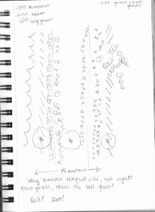
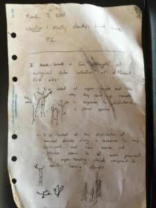
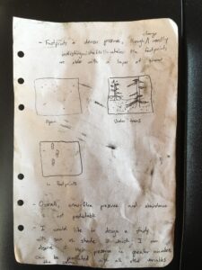
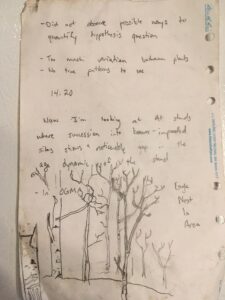
My study will be examining the incidence of White Poplar trees (Populus alba) relative to their proximity to the perimeter of their forested area. I noticed two different environmental gradients in my observations: (i) a north-south gradient and (ii) an east-west gradient. The north-south gradient is more pronounced, as the southern zone is abundant with coniferous trees while the north zone is absent of coniferous trees and contains various deciduous species (Figure 1). Since the distribution of trees close to houses has likely been manipulated by past owners, it would be difficult to be sure that my measurements are associated with ecological differences rather than anthropological differences (e.g., conifers would be attractive to plant near one’s home as they give more coverage/privacy in the winter months). For that reason, I will focus on the east-west gradient in the deciduous zone that I have identified. I have separated the deciduous zone into three subzones: (i) east zone, (ii) central zone, and (iii) west zone (Figure 2). The downslope from east to west is less than 10°.

Figures 1 and 2

2.

Observations:

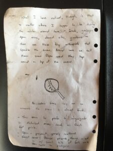
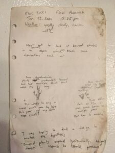
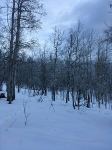
East zone: Abundant with various deciduous species that are native to Manitoba. White Poplar trees are more abundant on the north end of this zone. There were several large Manitoba Maple trees (Acer negundo L.) and Scrub Oak trees (Quercus macrocarpa Michx.). Coniferous trees were sparsely found in the southern region but decreased in abundance as I moved north, to the point of being absent at the north end. I could not reliably assess soil moisture becasue I had no equipment to do so and the snow had been melting over all of these areas over the last two days.

Central zone: Most diverse location and seemingly symmetrically distributed tree species. This zone, relative to the other zones, had a lower abundance of White Poplar that increases in abundance northwards. No conifers in the north end.

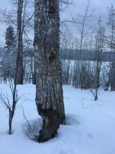
West zone: Appears to be the zone that is most abundant with White Poplars. Some conifers can be found on the south end, while none are found on the north end. The trees on the west perimeter seem to be uniformly slanted towards the west. The trees are approximately 5-10m from the adjacent dike which is currently dry. The overall

3.

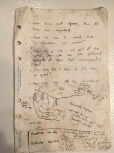
There are many factors that could be contributing to this gradient. Soil composition comes to mind as a potential contributor to the incidence of tree species. Sun exposure also probably plays a role. There seems to be much greater diversity and competition in the central zone, so the White Poplars may be competing with other tree species for sunlight. I believe that sun exposure would be a better “predictor” for White Poplars than soil composition, as White Poplars are hardy trees that tolerate an array of soil conditions. Furthermore, soil composition and White Poplar concentration may have a bidirectional relationship, whereas sun exposure and White Poplar concentration likely has a unidirectional relationship. Therefore, my proposed hypothesis is as follows.

Hypothesis: Sun exposure influences the incidence of White Poplar trees.

Prediction: The incidence of White Poplar trees will be greatest in locations of high sun exposure, like the east and west perimeters.

4.

Predictor (explanatory) variable: Duration of sun exposure (continuous)

Response (outcome) variable: Incidence of White Poplar trees (continuous)

A regression analysis would be sufficient for an experimental design (statistical analysis), as both variables are continuous.

Blog Post 3: Ongoing Field Observations

My study will be examining the density of coniferous trees in proximity to an adjacent creek (specifically Pinus ponderosa). The environmental gradient was chosen from the riparian bank to the upland forest apex, with three locations observed along the gradient; the riparian area, flood plain, and upland forest.

Observations were recorded in the field notes below, and in essence describe the density of tree species in relation to the area. It was observed that broad leaf deciduous trees dominate in the riparian area, with a noticeable lack of coniferous growth. The complete inverse was noted in the upland forest, with only Ponderosa pine inhabiting and a more diverse mixture of species in the adjoining flood plain.

I since formulated the hypotheses that the density of Pinus ponderosa decreases with proximity to Mission Creek within the observation area. A potential response variable would be tree concentration, while a predictor variable may be distance from riparian bank, or possibly the attributed soil conditions. These natural variables are both continuous, and would therefore justify a regression analysis.

Figure 1: Field notes (Loverin, 2021)

Observation 3: Ongoing Field Observations

1.With switching locations, I’ve really had to brainstorm what I could study at this location. I’m quite interested in birds, but also vegetation. Upon observing this location, I found it interesting how the vegetation differs on one either side of the raise footpath considered the dyke, and the sides of the dyke. I’ve scanned some images below to highlight how the growth differs on each side.

2. That being said, I chose three parts of the dyke. The first is along the water with the left slant of the hill, the top of the dyke pathway, and the right slant of the hill along the farm border. From the water to the farm border is about 15 meters with 5 meters in between each spot.

3. Besides the different proximities to the water, I observed that the soil seems to be a little different. Particularly on the bramble side (left side) it was quite rocky with less concentration of dirt. Perhaps this is why grass does not prosper along that side? I also observed that around 14:10-14:48 in the afternoon, the sun does not shine on the left side. In fact, it was quite cool without the direct sunlight. When you compare plot A to plot B, the sun is direct, there seems to be a saturation of water in the soil (there was mud present). Plot C also seemed to have some saturation in the soil (a little soft), but not as much as plot B. Surprisingly, because plot A is along the water, although on the hill, there was not a lot of water present. Is this because the water directly runs off the hill and into the water?

I’d like to explore a hypothesis about the soil composition and how it supports the type of vegetation that grows on each plot as well as the amount of exposure of sun throughout the day on B and C.


My formal prediction: The soil composition along the dyke determines the variety of vegetation that successfully grows in each plot.

4. The response variable for this hypothesis would be the vegetation and it would be a continuous variable. The explanatory variables will be the soil composition and amount of saturation that contributes to the soil composition. This will be a categorial variable. I will use a one-way ANOVA experimental design for this study.

Post #3 Ongoing Field Observations

I have looked at a few ideas for study options up to this point. Most of my experience has been in forestry and vegetation, so a vegetation-based project was my natural first choice. The fact that it is winter here in northern BC and the ground is under a few feet of snow is one reason why looking at something other than plants is maybe a good idea. Here are some of my ideas up to this point:

I thought of looking at shrub abundance in relation to conifer crown closure, but this would require a truly landscape-level study.

I thought of looking at beaver presence-absence as a predictor for shrub and aspen-ramet abundance, but once again this would require being able to see evidence of beaver which would likely be under the snow.

I thought of looking at pine plantations and observing how young individuals grow bigger and taller in the presence of nitrogen-fixing shrubs such as alder than those individuals growing where alder isn’t so abundant.

What I’ve finally settled on is something truly fascinating and present in so many different environments in these parts – an organism I see all around my home as well as in the forests that I walk, ski, snowshoe, and work in. I will number the following points as per the blog instructions in order to keep everything easy to follow.

1) We (my family and the people around me) call them snow fleas but they are actually springtails, tiny arthropods that present themselves in different abundances all throughout the winter. In the order of Collembola, they come out on warm winter days and jump around on the snow and their bodies contain proteins that act like antifreeze to allow them to function in sub-zero temperatures (wikepedia). I would like to study their abundance and distribution in terms of density under different circumstances.

2) I will describe three environmental gradients in which I’ve observed them:

  • Open undisturbed snow in which (as of today March 7 2021) they were fairly uniformly and sparsely distributed.
  • Forested ground with crown closure where I saw they were quite a bit more dense, interspersed throughout bits of tree debris and forest matter
  • Disturbed snow, particularly relatively fresh disturbances like footprints from a few hours prior before new snow has fallen, in which they seem to congregate in large numbers, sometimes on one side of the footprint or the other which begs a couple questions. Are they seeking shade within the disturbance? Do they just happen to be in greater numbers because the disturbance has decreased the snow depth in that one place?

3.) As far as processes that may contribute to their relative abundance in different circumstances – open, closed or forested, and disturbed – there are likely several reasons:

  •  As they are soil organisms, they are likely present in greater numbers over-top of ground that is richer or more nutrient-dense.
  • Snow-depth probably has a part to play – I would predict that as snow depth decreases, springtail density would increase.
  • Under cover of trees and with other bits of forest matter and debris scattered on the snow they would have more camouflage and be less visible to predators.
  • Direct or indirect sunlight may have an effect on their abundance.


One hypothesis I would like to explore – one that I think would lend itself to a study that would be possible to implement – is this:

Springtail density on the surface of the snow is determined by the presence of direct sunlight.

One formal prediction based on this hypothesis:

Though sunlight contributes to a warming environment conducive to springtail emergence, springtail density will be higher under cover or under a source of shade.

4.) The response variable in this case would be the density of springtails – this is a continuous variable. The explanatory variable would be presence or absence of direct sun (i.e. sun or shade) – this is a categorical variable. For this study, the experimental design would be a one-way ANOVA.

Blog Post 3: Ongoing Field Observations

The organism that I plan to study is the fern. I wonder what conditions ferns thrive, whether they grow better in sunny areas, semi-shaded areas, or shaded areas. The idea would be to look at the length of fern leaves and compare them across the different gradients.

I live on one side of a ridge and on my side where my house is, there is a large sunny yard, at the top it is semi-shaded, and on the other side it is completely shaded by old growth trees. The three locations along the gradient are the one area in my yard, which is near the top of the hill, and then following along the transect moving to a semi-shaded area at the top of the hill, and then moving along the transect down the other side of the ridge which is heavily treed. In the sunny area and in the shaded area there appear to be a lot of ferns, which are densely packed. Similarly, in the woods where there is no sunlight, there are similarly a lot of ferns. In the semi-sunlit areas there are also ferns, but not as densely packed. Having attempted to remove ferns from the yard, I observe that they are relatively tough. 

I hypothesize that the amount of sunlight positively impacts the growth of the ferns. I predict that the ferns will grow bigger in the sunlight areas because they thrive off more light. 

One potential response variable is the length of fern leaves and the explanatory variable is the amount of sunlight. The response variable is continuous and the explanatory variable is categorical meaning that it would be an ANOVA design. 

Post 3: Ongoing field observations at the Vancouver beach

My second field observation took place on the 20th of February, from 15:05 to 16:30, at multiple sites in the intertidal zone along the stretch of beach north of Volunteer Park. The weather was overcast and lightly spitting (it started raining more fully right after I finished), and approximately 7 degrees. High tide had been predicted at 10:34 (4m), and low tide was predicted for 18:34 (1.6m).

I initially wanted to compare oysters & mussels along the gradient from the top of the beach towards the water’s edge, by recording the number & size of all the oysters and mussels found in three spots from the beach’s edge to the water’s edge. I quickly realized after I started to make observations that the number of mussels, their sizes (ranging from 5mm to 90mm) and their close proximity to each other and attachments to various surfaces made this initial plan impractical. I decided to focus my observations on oysters instead, but because there were fewer oysters, I thought just three observations sites along the gradient might not be sufficient.

Ultimately I chose three locations along the beach – one at the stairs from Volunteer beach, the other two approx. 40-60m to the west and east of the stairs – and, starting right at the edge of the beach, I walked in a line towards the water. With each pace, I turned around and counted the number of oysters visible in the space between myself and where I had stood at the previous pace, within about 1 metre to either side (see the rough diagram in red, in the photos of my field journal). Each count was recorded in one square in my field journal, and I paced and counted until I ran out of space on the page. As I counted, I noticed that there seemed to be more oysters where there were big rocks (greater than ~30cm) than more “clear” areas, so I noted where there seemed to be more rocks as I was counting. In the third location, counting was hampered by the presence of seaweed/algae/general mud & slime that covered lots of the rocks and surface.

I want to focus on the distribution of the oysters, comparing areas with large rocks to areas without.

Possible processes that might cause the distribution difference:

  • large rocks provide more shelter, so in areas without shelter, the oysters are more likely to be predated upon by birds and therefore fewer would be found there
  • obviously since some of the oysters are not unattached, a large rock provides more surface area for oysters to attach, so more would be found there
  • possibly confounding factor: more attached oysters by big rocks might be competing for resources with unattached oysters, so more unattached oysters might be in places without large rocks

I hypothesize that the shelter provided by large rocks will cause more oysters to stay nearby. My prediction is that I will count more oysters, attached and unattached, very close to large rocks than I will count where there are no large rocks.

The predictor variable would be the presence of a large rock, which I would not control so it would be a natural, not a manipulated experiment. It is categorical, because it is either the presence or absence of large rocks. The response variable would be the number of oysters, which is a categorical variable, because it is a count of how many there are (contrast with if it was a measure of how big they grow, which would be continuous).

Post 3: Ongoing Field Observations

Ongoing Field Observations

What I plan to study are the variety or bird species and number of each bird species seen in three locations on this trail. I will observe species at the top of the hill on this trail. This is where the parch benches and feeders are, as well this is where there is a somewhat large clearing. I also plan to observe the species of birds present 100m from this point, as well as 200m from this point. I will observe the birds in terms of the variety of species, and how many of each species I observe within a set time. Each visit to the trail will be one hour. I will spend twenty minutes at each of these plots observing the species.

I hypothesize that the birds will be inclined to visit the feeders at the top of the trail, regardless of the larger number of people in this location. Therefore, I predict that there will be more species and a greater number of birds at the clearing at the top of the hill, than there will be at either of the other two test locations. I predict this outcome due to the bird feeders present, despite there being more people and less coverage  in this area.

A response variable within this study is the number of birds and variety of bird species that will be observed. This variable will be categorical, as it will entail the presence and/or absence of specific species. An explanatory variable would be the three locations which will be tested, and their proximity to the bird feeders, park benches, and forest clearing. This variable is continuous, as is can be measured by distance.

Blog Post 3: Ongoing Observations

For my study, I will be looking at western red cedars (Thuja plicata). For the environmental gradient, I focused on a gradient going from no trees of any species to abundant cedar trees.

The first location had no trees of any species. It was a rocky meadow, where there is very little soil on the surface of the bedrock. The bedrock is mostly covered in a layer of moss that is about 3.7 cm thick  with occasional patches of completely exposed bedrock (see photos for data and species – this data will not be used for my study as the thickness of the moss is dependent on its species but I thought it would be interesting to include it in my description here). The most common moss present was Oligotrichum parallelum. This location had the most moisture of the three locations I observed on the gradient. Water pooled around my feet as I stepped on the moss and there were small puddles in the depressions of the rock.

The second location was on soil with a layer of moss about 6.6 cm thick. The most common species of moss was Kindbergia oregana and there is not a single patch of exposed soil. This location had lots of other low-growing plants, arbutus trees and Douglas fir trees, but no cedar trees. This location was less moist than the last, but still moist enough that my feet would’ve gotten wet if they were not already.

The third location had thinner, more patchy moss and there isn’t a dominant species. There are many sections of exposed soil and lots of debris from fallen branches. I observed 10 living cedar trees from where I was standing and many more that were dead. Moss did not grow at the base of the living cedars but it was much more common at the base of dead cedars. This location was the driest, as it didn’t have as much moss to hold water. My feet would’ve stayed dry if I had stayed in this location!

My hypothesis is “The distribution of Thuja plicata is affected by the biomass of moss present.” and I predict that “Both Thuja plicata and a large amount of moss will not be present in the same location.” The response variable for this study is the presence of cedar trees and the explanatory variable is the biomass of moss. The response variable is categorical and the explanatory variable is continuous.

Link for the photos (I apologize for the slightly blurry parts):

https://photos.app.goo.gl/vAx3R94qfCTjG77w8

Post 3: Ongoing Field Observations

1) I plan to investigate the presence of green trunk pigmentation in aspen trees. I would like to determine if it is present on all aspen trees or if there are factors affecting the distribution.

2) My initial observation area only contained one small stand of aspen trees. Since aspen trees in close proximity to one another are often clones of each other, aspen trees from other areas would need to be observed in order to have independent replicates. I chose five different areas to observe aspen trees. The distance between the areas ensures the populations were independent of each other. Once I arrived at an area, the trees were chosen haphazardly mainly due to accessibility. I also had to choose areas that were accessible at this time of year by car as well as areas that had trees in snow shallow enough to be accessed on foot. Since accessibility was a concern, all the sample areas were located in close proximity to roadways or plowed parking lots.

In my first sample area I observed that the green color was present on the south east side of the trees but was not visible on the remainder of the trunk circumference. I observed three trees in this location and found them all to have the same green distribution pattern. The trees in the first area were in an open field on the edge of a cliff above a riparian area and had no competition for light or nutrients. Based on the observations from the first area, I wanted to see if different levels of competition/vegetation type, elevation, or direction had any impact on the presence of the green color.

The second area I observed was approximately 1.5 km from the first. The vegetation in this sample area was populated with both coniferous and deciduous trees. This type of vegetation provided much more competition for light and nutrients than was present in the first area. Five trees were observed at this location and all had green pigment present. The coloration was observed to be mainly on the south east sides of the trees and didn’t start until approximately three feet up the tree. Two of the trees were in denser areas of the forest and the green color was observed to be all the way around the trunks on these two trees. The bark on the larger, older trees was not green on the north side since this side is typically very rough and black so green pigment would not be visible.

The third area was the furthest away and the highest elevation. The trees in this area were again in a forested area with competition as well as being in a harsher environment due to the elevation. Winter in this area typically lasts longer and has much more snow than the other areas sampled. All the trees sampled in this area were green all the way around the trunk. One tree on the edge of a clearing had darker green coloring on the north side of the trunk. This tree was on the edge of a small clearing and had no immediate competition on the north side.

The fourth area was similar in climate to the third area but the trees in the fourth area were in the open with minimal competition. The trees with the smaller circumference in this area were found to be green all around and for most of the height that was observable with the south east side being a darker shade of green. The larger trees were a much lighter shade of green. One of the trees sampled in this area was next to a light that came on at dusk and off at dawn. This tree had very limited green visible.

The fifth area was on the edge of a marsh. The trees in this area were in the open with no tree competition and plenty of access to resources. They were located in town so may also have be impacted by artificial light. The green on these trees was noticeably darker on the south west side of the tree. The trees in this area did not have black scabby bark on the north side and they had branches growing almost uniformly on all sides. The trees in this area were observed to have green pigment present on their branches as well.

3) The patterns I observed could be caused by competition from surrounding vegetation, access to sunlight, exposure to artificial light, age of tree, or elevation.

My hypothesis is that green pigment will be present on the south side of all aspen trunks. I predict that the aspen trees will have green pigment on the south side of the trunk to maximize its access to sunlight.

4) One response variable is the presence of green coloring on the trunk of the aspen tree. An explanatory variable would be surrounding competition for sunlight. In this experiment the response variable would be categorical and the explanatory variable would be continuous.

Post #3 Ongoing Field Observations

I initially went out to my field site with the hopes of finding patterns in the way shrub species such as Amelanchier alnifolia and Salix were responding to browse pressure by moose. Looking at percent cover of biomass, horizontal growth patterns, or length of new shoots, I wasn’t able to imagine a study design that could answer specific questions, or maybe I just couldn’t formulate questions that lended themselves to good scientific study.

Thoughts on browse patterns

So I moved on to several places around my lake where Aspen stands have sent out suckers following beaver disturbance that ended some time ago, observing the gradient between the older stand and the younger individuals that have come up.

I also noticed other places where aspen were encroaching on fields or human-cleared sites, and some of these had distinctive successional gradients, too. And now to come up with a study design:

Aspen succession observations

1.) Identify the organism or biological attribute that you plan to study.

I plan to study Aspen trees in the process of succession.

2.) Use your field journal to document observations of your organism or biological attribute along an environmental gradient. Choose at least three locations along the gradient and observe and record any changes in the distribution, abundance, or character of your object of study.

One location is inside the parent clone of the aspen organism, where the individuals are mature with similar ages (presumably) and similar sizes (heights and diameters). Also noteworthy may be variables such as density, basal area, and incidence of health or pathological indicators such as conk.

Transition between aspen parent and offspring

A second location along the gradient is where there is an obvious shift in the clone’s attributes such as size, age, and density; i.e. where the aspen clone initially sent out suckers in response to the disturbance from years ago, and there is a higher abundance of individuals.

The third location along the gradient is the point at which there are no longer any suckers coming up, or where the suckers are obviously young or new clones, and maybe more abundant. In some places, shrub species are present in varying numbers/densities at this point on the gradient with varying levels of browse, and some of the aspen suckers are also being affected by browse pressure. Could the aspen be responding to browse pressure by continually putting out new suckers?

3.)Think about underlying processes that may cause any patterns that you have observed. Postulate one hypothesis and make one formal prediction based on that hypothesis. Your hypothesis may include the environmental gradient; however, if you come up with a hypothesis that you want to pursue within one part of the gradient or one site, that is acceptable as well.

Several processes are likely acting on the aspen trees to cause differences in the way they expand and fill the spaces they occupy following disturbances. Aspect, slope, and time are definite variables influencing the rate of aspen expansion I would think. I’m also curious about how the age and density of the parent stand at the time of clonal expansion influences how the younger clone individuals proliferate/spread. Many potential hypotheses to pursue…this project may incorporate the Hypothetico-Deductive Method approach.

I think I’ll start with age of the parent stand influencing how the younger clones develop. I hypothesize that the older the parent stand, the less its offspring will spread, or the less biomass will be produced by offspring. Framed another way, I hypothesize that the younger and “more vigourous” the parent stand is, the denser (or taller or further-travelled) the offspring will be.

4.) Based on your hypothesis and prediction, list one potential response variable and one potential explanatory variable and whether they would be categorical or continuous. Use the experimental design tutorial to help you with this.

Response variable: Density of the younger aspen. Or height to age ratio of younger aspen. This is continuous.

Predictor variable: Age of the parent stand. Though ascertaining the age of multiple trees would provide a continuous dataset, in this case (because aspen are clones) the parent stand’s age may be categorical, e.g. “veteran, mature, older immature” etc.

If I were to predict that offspring density or site index (a continuous variable) would be affected by the parent’s age as categorical, the statistical design would be ANOVA.

If I were to predict that offspring density or site index (a continuous variable) would be affected by the parent’s age in years (or density, basal area, site index – continuous variables), the design would be a regression analysis.