Blog Post 3: Ongoing Field Observations

For my ongoing field observations, I visited Pipers Lagoon on Sunday, January 17th at 9:43 am.  The weather was overcast, 6 degrees in temperature, and no wind.


1. Identify the organism or biological attribute that you plan to study.

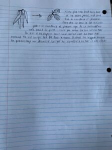
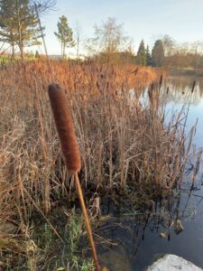
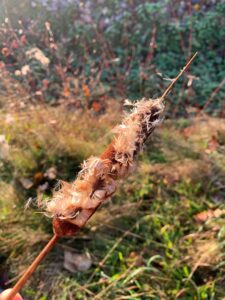
The organism I plan to study is the Broad-Leaved Stonecrop, sedum Spathurifolium.


Figure 1: Broad-Leaved Stonecrop

2. Use your field journal to document observations of your organism or biological attribute along an environmental gradient. Choose at least three locations along the gradient and observe and record any changes in the distribution, abundance, or character of your object of study.


During my first field observation, I had noted that the Broad-Leaved Stonecrop was generally only found along the ocean-facing rocky outcrops and not present on the lagoon facing ones. The plant is able to grow within various cracks and crevasses in the rocky outcrops. During this field observation, I decided to use the elevation from sea level as my gradient as well as exposure to the sun and the ocean. I also decided to focus on just the headland island portion of the park. 

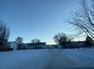
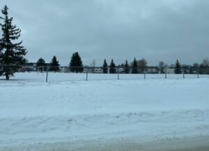
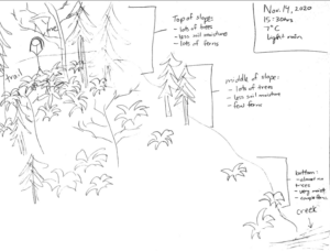
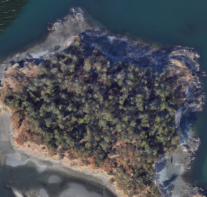
I chose three different locations along the headland island, all with similar topography (open, exposed cliffs, primarily moss/lichen/stonecrop dominant). These were the northeast rocky outcrop, northwest rocky outcrop, and the south/southwest portion of the headland island. 

Figure 2: Observation Locations

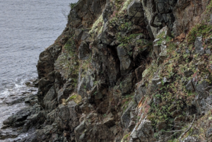
Along the rocky outcrop of the northeast side of the headland island, the stonecrop generally grew from mid to high elevation from sea level, with no growth at all below the high watermark. It was typically most abundant mid to high elevation, with less abundance along the plateau. As the amount of sun exposure throughout the day differed (i.e morning vs afternoon) it was noted that the abundance and distribution of the stonecrop increased (i.e more abundant and more area covered along the west side of the rocky outcrop than the east). Again, the growth was most pronounced at mid to high elevation and tapered off along the plateau. It was also noted that the stonecrop more exposed to the sun throughout the day had a more reddish color to its leaves than those that were in less sun-exposed areas.

The northwest rocky outcrop of the headland island had a similar growth regime (i.e mid to high elevation, tapering off at the plateau). It was noted that the stonecrop distribution spread beyond strictly the rocky outcrop on this portion of the headland island. A large abundance was observed along a steep slope farther inland than the rocky outcrop.

The Southwest portion of the headland island had virtually no presence of stonecrop, despite being a similarly rocky, sun-exposed area. However, there was certainly more soil and much less hard rock here than the more sea cliff type rocky outcrops in the other areas. This area also has no exposure to the open ocean while elevation gain from sea level was much more gradual and smaller than the much sharper increase in northeast and northwest portions of the headland island.


3. Think about underlying processes that may cause any patterns that you have observed. 


Some underlying processes that may cause the patterns observed include the moisture and drainage of the substrate that the stonecrop grows in, the type of substrate, and the amount of sunlight exposure.

Postulate one hypothesis and make one formal prediction based on that hypothesis. Your hypothesis may include the environmental gradient; however, if you come up with a hypothesis that you want to pursue within one part of the gradient or one site, that is acceptable as well.

Based on my observations of where the stonecrop was found to be thriving I hypothesize that stonecrop abundance is negatively impacted by increased substrate moisture. Therefore I predict that the stonecrop will be most abundant in areas with at least half-day sun exposure and bare, exposed rock.


4. Based on your hypothesis and prediction, list one potential response variable and one potential explanatory variable and whether they would be categorical or continuous. Use the experimental design tutorial to help you with this.


One potential response variable would be the abundance of stonecrop while one potential explanatory variable is substrate type. Substrate type would give an indication of the amount of moisture the stonecrop is exposed to as well as the drainability of water in the area. The response variable would be considered continuous (i.e abundance in terms of percent cover) while the predictor variable would be considered categorical (i.e type of substrate). This would classify the experimental design as being ANOVA.
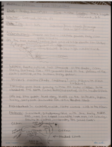
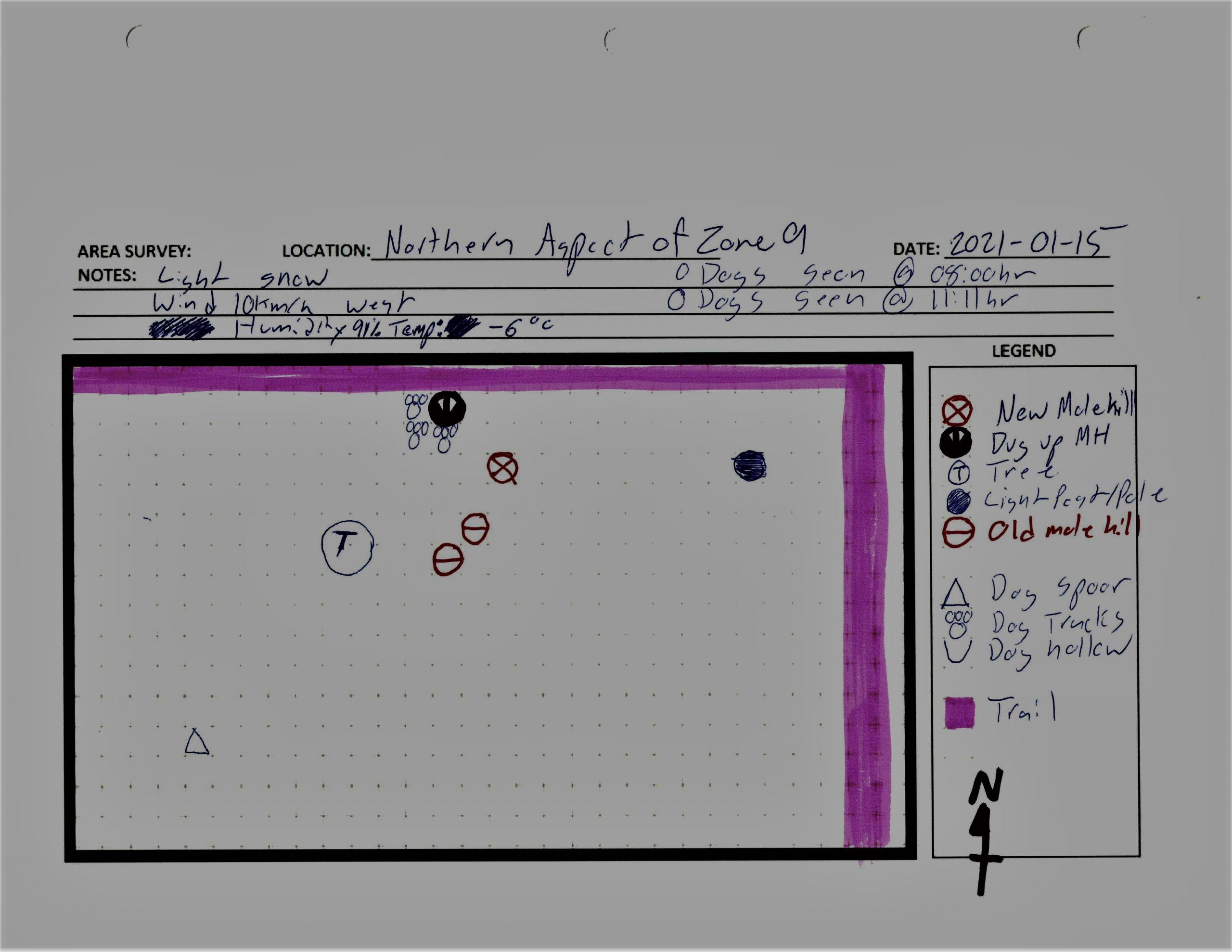
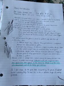
Field Notes:


Blog Post 3: Ongoing Field Observations

For the course project I have been gathering data on the ecology and communities of a 1km x 1km area in western Ukraine.  The following information contains both my ongoing field observations and my considerations regarding a possible hypothesis.

Organism or Biological Attribute:
For the course project I have chosen to study the Eastern European Mole, and how it interacts with local predators such as dogs and cats.

Documentation:

I have been observing and documenting mole colonies, dog sightings, cat sightings, weather conditions, and mole hill activity over the last month in the observation areas. Specifically Zone 9, Zone 15, Zone 12, and zone 7.  Contrasting to this, there is a single Zone I have been documenting called ‘Control zone’ east of the observation area which has no Canine or Cat activity observed.

Example of Zone observations

Gradients Observed:

TOPOGRAPHY: In the control area, there is a gradient of topography with approximately a linear grade from the southern aspect dropping approximately 12 feet to the northern most aspect. Of note there is approximately an 8 foot gully near creek on western aspect of observation area.

VEGITATION: The general area which the moles are observed is the grassed areas which sit on a sandy aggregate soil.

PREDATORY CONCENTRATION: There appears to be a higher concentration of predators in north western aspect of observation areas, but less in south eastern area either due to topography,  territorial behavior, access to food, or a combination there of.

GROUND: Keeping in mind soil types change throughout the area. Again, the mole hills appear in sandy soil but the depth gradient of tunnels is not able to be directly observed despite the research on moles that indicates that these can go as deep as 6 feet. There is a carpet of decomposing leaves and rich soil under the oak trees (often thick with acorns) but little to none under pine trees.

TEMPORAL: Over time the count of active mole hills, spoor, coil conditions, and weather changes which may affect activity levels of all organisms in observation area.


Three locations inside the Observation area are:
——————————–
North west aspect of Zone 9 – Medium to low dog activity in area/transit point no sleeping
Northwestern Aspect of Zone 15 – Low dog activity in area as they adhere to eastern aspect for midday sleeping.
South eastern aspect of Zone 7 – High Dog activity due to transit+sleeping area
Central area of Zone 12 – Low mole hill count, high dog activity during midday.
Control area: Zero dog/cat activity – Zone A (east of map)

Area of Observation
Area of Observation

Processes and Patterns

Anecdotally the mole hills appear more populus and active in zone 9 and 15, as well as the control area to the east. This seems to be inverse to the dog activity in those areas. The temperature changes over time seem to affect the mole activity to some extent.

Hypothesis

The number of predatory dogs and cats in the area directly effects the activity of the colonies in the observation area.

Response variable(continuous): Mole hills along the gradient of dog activity.
Explanatory/Predictor variable (continuous): Number of dogs in the area (based on sightings and new signs)

Initially this appears that a study for this hypothesis would be of a regression design


Blog post 3: Ongoing Field Observations

Nov 22nd          Time: 1:30pm             Temp: 40C       Weather: Windy with overcast

Some of the dominant evergreen trees in Kenna Cartwright park are Douglas fir and Ponderosa pine. This project will be focused on the distribution of the evergreen trees with respect to the distance from the entrance point of the park.

These trees are easily identifiable, they have needle-shaped leaves, compared to the deciduous vegetation in the area that have lost their foliage.

Five different distances between 0 – 1000m were selected at which 50 x 5m belt transects were taken at the 5 different locations. These 5 distances were predetermined by an online number generator.

My prediction is that the density of the trees will increase the farther away from the entrance point. This may be due to the decreased human activity with an increase in this distance.

The response variable is the density of the trees and the explanatory variable is the distance from the entrance point to the park; this point is considered the zero point of measurement.

Since both of the variables are continuous, the regression experimental design will be utilized.

Blog post 3 images 

Instructor: Robyn Reudink

Blog post 3

I watched my chosen area on Jan 5th, 2021 throughout the day from my garden. I decided to conduct my field research study on the presence of white-tailed deer. Specifically, the distribution and number of them across the three locations I identified along the environmental gradient.

The 3 locations I chose were as follows: open field, city road and residential area. The deer did not venture into residential, however, in the other locations, they tended to be present.

Deer’s travel in a herd to protect against potential predators.

My prediction is that the open space has the most vantage point to observe any potential threat and therefore they would most likely aggregate in this area.

One potential response variable is the number of deer (continuous)One potential predictor variable is the amount of access to the open field without the presence of a threat (categorical).

Based on the experimental design tutorial my experimental design would be classified as ANOVA

Post 3: Ongoing Field Observations

Identify the organism or biological attribute that you plan to study.

The organism I will observe is the presence or absence of the Parthenocissus quinquefolia, more commonly known as the Virginia creeper. 


Use your field journal to document observations of your organism or biological attribute along an environmental gradient. Choose at least three locations along the gradient and observe and record any changes in the distribution, abundance, or character of your object of study.

I visually divided my observation area into three transects; the areas include a clear cut section where sand has been spread to form a makeshift road, a small area where regrowth is forming that had been selectively cleared, and an area that has only been affected by natural treefall.  Changes of the Virginia creeper along the gradient includes the abundance, having a larger presence in the old-growth area than in the regrowth area or on the sandy road. The size of the Virginia creeper also differed. In the old-growth area there were many clumps and expanding vines, in the regrowth area there were smaller clumps with a few vine shoots, and finally, on the makeshift road there were fewer smaller clumps few big enough to shoot vines.


Think about underlying processes that may cause any patterns that you have observed. 

Underlying processes that may cause patterns in my observations include differences in soil nutrients as well as different compositions resulting in the inhibition or deterrence of Virginia creeper to grow. On the makeshift road and regrowth area the size of the Virginia creeper plants and their density could be smaller because there is greater anthropogenic activity, the sand adds an extra layer of soil to grow through, and plants haven’t had as much time to regrow in these areas. 


Postulate one hypothesis and make one formal prediction based on that hypothesis. Your hypothesis may include the environmental gradient; however, if you come up with a hypothesis that you want to pursue within one part of the gradient or one site, that is acceptable as well.

My hypothesis is plant richness of Virginia creeper is negatively affected by anthropogenic activity.

One prediction is that the plant richness of Virginia creeper will be more abundant in areas with less anthropogenic activity.


Based on your hypothesis and prediction, list one potential response variable and one potential explanatory variable and whether they would be categorical or continuous. Use the experimental design tutorial to help you with this.

The response variables in the experiment included the absence or presence of the Virginia creeper. Given that the dependent variable(the presence or absence of Virginia creeper) is dichotomous, categorical I would test the hypothesis using logistic regression. The predictor variable is the locations (also a categorical variable).  This is a categorical logistic regression design as the observation is to determine the overall presence of Virginia creeper growing in each transect.

Post #3: Ongoing Field Observations


  1. Identify the organism or biological attribute that you plan to study. Canadian Geese 
  2. On the grass: every goose is more spread out from one another. Their distribution is more spread out and everyone is picking at the grass, looking for something to eat. There are a lot ~30 geese presentBy the trees: in the summer months the geese were either under the trees or some of them were in the sun (sunbathing). they were always in groups thoughOn the lake: only a few left the group to go to the lake but they always go in groups. Around 6-7 of them were present on the lake and they peck at the water at first and stood by the riverside and then eventually went in the lake with some of them swimming and some still on the edge.

  3. Think about underlying processes that may cause any patterns that you have observed. A: All of the geese stay in pairs, even though they may be spread out from another, they are always together.  Postulate one hypothesis and make one formal prediction based on that hypothesis. Hypothesis: What is in the habitat of Canadian Geese that causes them to gather in large numbers? What food sources do Geese look for on the grass?
  4. Based on your hypothesis and prediction, list one potential response variable and one potential explanatory variable and whether they would be categorical or continuous. Use the experimental design tutorial to help you with this.

Response Variable: Which foods are rich in grasslands that cater to the diets of Canadian Geese.

Explanatory Variable: The types of food sources available. (Categorical)


Post #3 Ongoing Field Observations

I have continued to do field observations in my area of study. One my last visit, I identified two very interesting phenomena that did not catch my attention the last few times I have been there. I am not quite sure which experiment I am going to choose, so I am going to write this post inclusive of both of them and perhaps with some feedback and further consideration I will come to a final decision.

Option One:

I may choose to study the cottontails that surround the pond. There is a large amount of them in varying abundance in different groups around the pond. During my last visit, I noticed that some of the cottontail heads are beginning to fall apart, which I assume is for reproduction similar to how dandelions reproduce because they seem to fall apart into white fluff that seem like seedlings. However, some groups have many cottontails that have fallen apart or began to fall apart easily upon some light shaking and tapping with a stick. Other groups in the pond had cottontail heads that were still very firm and remained that way with similar shaking or tapping. After considering variables such as cottontail height, sunlight, cottontail abundance, and moisture, there did not seem to be any patterns. I later realized that I was not taking into account the pine trees as part of the abundance, and noticed that it seemed that the more crowded an area was, the less likely it was to have cottontails that were falling apart. I hypothesize that the cottontails that have less vegetation nearby and therefore less competition fall apart and reproduce faster, ensuring them better success and fitness, because they have better access to the available nutrients in the ecosystem. My prediction is that cottontails in less crowded areas would fall apart earlier and cottontails in more crowded areas would fall apart later in the season. Possible response variables could be the degree to which the cottontails have fallen apart (continuous) or the ratio of cottontails that have fallen apart versus stayed intact (continuous) and the possible explanatory variable could be number of cottontail heads in a given study area (continuous), number of trees and distance from the identified group of cottontails (continuous).

Option Two:

As I noticed the role of the pine trees in this pattern with the cottontails, I saw that they were in the process of making and dropping pine cones. Some trees had many early pinecones and some trees had many late stage pinecones in a way that varied greatly from tree to tree. I thought perhaps that they followed a similar pattern as the cottontails in terms of crowding and competition, but this did not seem to have any recognizable pattern. However, because this visit was done during clear skies, I was able to see how the sunlight hit the trees for most of the day and the path it would take across the sky over the daylight hours. That is how I noticed that the trees that got more sunlight seemed to have more early stage pinecones and the trees blocked by the shade of other trees as well as the branches that got less direct sunlight had more of the late stage pinecones. I hypothesize that decreasing sunlight is a trigger that signals to the plant that it is winter and time to shed the non-useful parts of the tree, triggering the shift from early to late stage pinecones. I predict that the trees that receive the most direct sunlight will shift into late stage pinecones later in the season that those that do not receive as much direct sunlight. The response variable would be the ratio of early to late stage pinecones (continuous) and the explanatory variable would be sunlight amount (low light versus high light) (categorical).

Blog Post 3: Ongoing Field Observations

The organism I plan to study for the field research project is three types of large forest trees, the western red cedar, the ponderosa pine, and the Douglas-fir tree, within the Woodhaven Nature Conservancy Regional Park.

The trees change along an environmental gradient.  The first location (Figure 1) has many western red cedar trees and is dense with trees (Figures 2 and 3).  The location is shady with lots of dead fallen trees.  The ground cover are plants with dark green leaves; this seems to occur where there is sun exposure.  Much of the ground does not have plant growth due to the shade.  The distribution seems somewhat even.

The second location (Figure 4) is up a steep incline where the main tree is ponderosa pine (Figures 5, 6, and 7).  The soil appears sandy and the ground cover is more grass-like.  These trees are sparse and less dense than locations 1 and 3.  The distribution appears more uneven than locations 1 and 3.

The third location (Figure 8) is densely populated with Douglas-firs but is less dense than location 1 with the western red cedars (Figures 9 and 10).  The ground cover is a mix between grasses and the shrubs with dark green leaves.   The distribution appears even.

An underlying process which may cause the changing of the dominant tree type pattern could be changes in elevation which could influence soil moisture. My hypothesis is elevation influences the types of large trees that grow within a forested area.  My prediction is the first location with the western red cedars has the lowest elevation, the second location with the ponderosa pines has the highest elevation, and the third location with the Douglas-firs has an elevation in between the first and second locations.

The response variable would be the tree type (western red cedar, ponderosa pine, or Douglas-fir) that is growing within an area of the environmental gradient and the explanatory variable is elevation.  The tree type is categorical as the three trees I’m interested in are western red cedars, ponderosa pines, and Douglas-firs and if they are present or absent at different elevations.  Elevation would be continuous as it is measured on a continuous numerical scale.

Post 3: Ongoing Field Observations

I visited the ravine again on November 14th at around 15:30 hrs. It was a cloudy day again with some light rain and a temperature of 7°C. I decided to focus my observations on the ferns this time and also chose the slope as my environmental gradient. From my research, I was able to identify the species of ferns as Polystichum munitum, or the western sword fern. I also took a different route at the top of the ravine to get a different view and to see if I still noticed the pattern of the ferns being more abundant higher up and away from the creek. 

At some points along the trail, there was not a noticeable difference in the abundance along the slope. However, at many areas, I could see that were many more ferns at the top compared to the bottom. I was able to confirm the pattern I saw last time. I stopped at one point along the trail and chose three locations on the slope to study the ferns: at the bottom right by the creek, halfway up the slope, and then near the top of the slope.

Bottom of slope: very moist soil, not many trees, only 3 ferns

Middle of slope: soil a little less moist than bottom, lots of trees, maybe 5-7 ferns

Top of slope: soil a little moist, lots of trees, lots of ferns

There could be many possible reasons to explain this pattern including, soil moisture or water content and sunlight exposure. I know ferns tend to grow in damp, shaded areas, so moisture and sunlight exposure are definitely factors that I can explore as possible reasons for my hypothesis.

Based on my observations I have come up with a hypothesis, prediction, response variable, and explanatory variable.

Hypothesis: Creek proximity affects Polystichum munitum abundance.

Prediction: As distance from the creek increases, Polystichum munitum abundance increases.

Response Variable: Fern abundance (continuous)

Explanatory Variable: Distance from the creek (continuous)

Field journal entry from my visit showing the fern distribution along the slope

Post 3: Ongoing Field Observations

For my research project I am going to look at population density and vegetation abundance from different intervals and elevations from the stormwater pond in Fish Creek.
I am going to be looking at the abundance of cow parsnip, common yarrow, silver sage and veiny meadow rue.
I have initially noticed that there is a clear distinction in vegetation abundance along the stormwater pond and maybe this could be the normal floodplain for the pond when it experiences a flooding situation after a rainfall.
I am going to look at 4 distinct areas and see if there are noticeable differences in vegetation species and densities based on the amount of flooding experienced.
Area 1: an area immediately next to the stormwater pond which is classified s a natural wetland. This leads me to believe that the vegetation and landscape has not been or at least minimally altered by humans.
Area 2: a riverine area located at lower elevation and closer proximity to the stormwater pond.
Area 3: a riverine area located at higher elevation and further away from the stormwater pond and right beside the walking path.
Area 4: a grassland area located at higher elevation and with the walking path creating a barrier between the grassland area and the stormwater pond
My hypothesis is that the stormwater pond, the frequency of flooding and the floodplain average height will determine the species and abundance of vegetation growing in Fish Creek.
I’m predicting that cow parsnip will be more prevalent at lower elevations as it is more resilient and species such as the veiny meadow rue will be more abundant at higher elevations that experience less flooding.
An explanatory variable could be the distance from the stormwater pond and how much water vegetation is receiving. A response variable could be the abundance of vegetation present if there is any in certain regions.