Post 3: Ongoing Field Observations

I plan to study Peterson Creek as a viable spawning area for salmon and the effects of the aesthetic grooming of the creek could be having on that population.

The three locations I chose as my sample areas were at the base of the waterfalls where I noted the finest sediment and largest girth in the stream bed. I observed the gradient of the falls and levels to it, ensuring it was possible for fish to travel from the feeding lake above.

 I then traveled 0.5 kilometers downstream where I had first observed red algae along the edges of the stream indicating a food source and nutrients to sustain fry growth before entering the Thompson River. The rocks were much larger in this part of the creek and the water was much shallower while the walls of the stream were narrow and steep compared to the gradual gradient and deep pools found at the base of the falls.

The final location I chose was the beginning of the park another 0.5 kilometers downstream to see the most heavily traveled portion of the creek. This area has evidence of heavy travel in and around the water by dogs. There was absolutely no visible plant life in the water and around the creek bed was only grass, no shrubs which indicates heavy travel in the area. There were bits of garbage littered  around the tree bases.

The frequent creek bed disturbance by human intervention through methods of removing debris has resulted in the area being uninhabitable for local fish.

The areas of the creek with adequate substrate and width for fish to lay eggs shows evidence of removal of debris. This area will have depleted biodiversity and few if any fish inhabitants.

Based on my hypothesis, the response variable is the salmon population, it is considered categorical. I aim to measure their presence in the creek. The explanatory variable I have identified based on my hypothesis is the people who visit the park. It is considered categorical as I will be measuring their influence on the creek’s biodiversity.

Post 3: Ongoing Field Observations

The fieldwork began by proposing simple research questions and developing a hypothesis and evaluating using scientific literature. The fieldwork used different light traps to sort and identify the insects’ orders by employing simple diagnostic keys. Insects are important components of biodiversity, and therefore it is important to understand and appreciate the several roles of the insects in the ecosystem. Their interesting natural history well shows the benefits of the insects in the ecosystem. Hence facilitates the application of the insects as models of learning the ecosystem conservation.

Blog post 3, Ongoing Field Observations

Attribute:


The attribute I have chosen to study is the health of perennial streams found in rangeland areas. I specifically noticed that there was disturbance to the stream bed and presence of invasive thistles in riparian zones at locations that the cattle had easy access to.


Observation:


I have observed locations at three points along one perennial stream (Figure 1).  The locations include an area with strong evidence of disturbance by cattle, an area upstream from the disturbance, and an area downstream from the disturbance.  The locations upstream and downstream were chosen by accessibility to the locations. I have also observed two other stream locations along a perpendicular gradient that are easily accessed by cattle.  I have found that the slope of the banks and access to the stream to be the biggest indicator for possible deterioration of the health of the stream.  The locations that have easy access, those along the perpendicular gradient, have evidence of disturbance causing changes in the stream bed (Figure4) and the presence of Cirsium vulgare (Figure 2), and Cirsium arvense (Figure 3). These observations areimplications of decreased health of the stream.  The areas along the gradient of the single stream indicate that the impact of the cattle is limited to the areas they can directly access.


Pattern:


The pattern I have observed is that there appears to be deterioration of the streams, stream beds, and riparian zones in small perennial streams in rangelands at points of low slopping access. The stream beds are highly disturbed and are no longer gravelly in appearance.  In these disturbed areas the stream bed has become muddy; further, invasive thistles are present in these disturbed areas.  A possible process that has caused this deterioration is cattle accessing the stream. This is particularly evident in areas of easy access due to low sloping approach to the streams.


Hypothesis:


The ability for cattle to access perennial streams in rangeland with low sloping access points is contributing to deterioration of the stream health in areas directly accessed by the cattle.


Prediction:


The stream will show diminished overall health in areas that show high disturbance and presence of invasive thistles.


Variable example:


One response variable to study would be the presence of invasive thistle, specifically Cirsium vulgare, it could be categorical and measured in presence absence.  The potential explanatory variable would be that cattle are contributing to the spread of the invasive thistles shown by the presence of the thistle in areas accessed by cattle.

Figure 1 Field journal observations


Figure 2 Cirsium vulgare
Figure 3 Cirsium arvense
Figure 4 Disturbance by cattle


Blog Post 3. Ongoing Field Observations

The organism I am interested in is scentless chamomile (Tripleurospermum perforatum). Scentless chamomile is abundant on top, but is almost absent at the bottom of the pits.
My locations to record are:

1. On top of the mineral soil: Here the scentless chamomile is the most abundant and tall.

2. Mid-way down the slope: There is a steep decline in the abundance of scentless chamomile mid-way between the topsoil and the bottom of the pit.

3. The bottom of the pit: There is almost no scentless chamomile at the bottom of the pits.

I hypothesize that areas with abundant scentless chamomile will not be acidic. The explanatory variable would be pH (continuous) and the response variable would be scentless chamomile abundance (also continuous). I will measure the pH along the gradient to determine where it is high and where it is low and measure the abundance of the scentless chamomile to compare.

Post 3

Blog#3

Field Research Project

Blog Post 3: Ongoing Field Observations

Create a blog post to document your ongoing field observations. Supplement your blog entry with scanned or uploaded examples from you field journal. Specific points you need to cover are:


  1. Identify the organism or biological attribute that you plan to study.

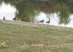
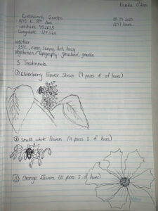
I plan to study poison ivy distribution in a disturbed habitat.


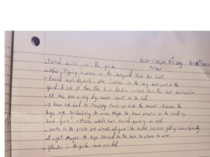
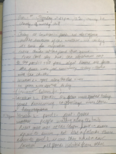
  1. Use your field journal to document observations of your organism or biological attribute along an environmental gradient. Choose at least three locations along the gradient and observe and record any changes in the distribution, abundance, or character of your object of study.
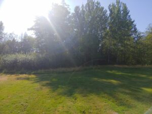
 

Location 1

meadow

Location 2

forested

Location 3

old field

Distribution none Clumped Clumped
Abundance 0 3 4
Character none Low growing some climbing


I visually broke up the area into three zones and followed a transect line along the edge of the trail. I recorded for 1 meter x 1metre plots just off the trail at the start of each zone. The meadow begins at the start of the trail. The forest begins at the same spot on the other side of the trail and the field begins where the forest thins and I can see the open field through the trees.


  1. Think about underlying processes that may cause any patterns that you have observed.


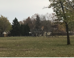
Other trails in the area, including one only approximately 0.5km down the road did not have any noticeable poison ivy present. This had originally led me to wonder if the heavy equipment presence had anything to do with the abundance on the trail I am researching.

I reviewed research indicating that poison ivy will grow well in disturbed areas, so that may be a factor in why it’s doing well on that trail (Admin, 2016). I still wondered however why the distribution of the poison ivy is concentrated on the left side of the trail, especially since the right side is more disturbed. I had thought that shade may be the factor, however my research indicated that poison ivy does well in both shade and sun, so I don’t think that is the main explanatory variable (Admin, 2016).

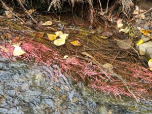
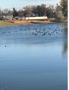
After completing the table above, I noticed that the plants tended to grow in clumps, rather than as individuals spread out. The clump in the forest location was growing amongst raspberry bushes and the field clump was climbing up a rock, near an apple tree. There were several species of birds including crows, chickadees, and woodpeckers that I noted. There are many mammals as well such as deer and chipmunks which I have encountered on other walks. According to Brown, several animals eat poison ivy and distribute seed. I am wondering if foraging sites like the apple tree and raspberry bushes will have a higher poison ivy concentration overall. This could be due to dropping seed while feeding (Diane Brown 2018). In fact, I saw a chickadee relieve itself while perched on a tree just a little further down the trail. Another place that I have noticed poison ivy is in the lot next to me. There is an apple tree there, which adds to my suspicion about a connection.


  1. Postulate one hypothesis and make one formal prediction based on that hypothesis. Your hypothesis may include the environmental gradient; however, if you come up with a hypothesis that you want to pursue within one part of the gradient or one site, that is acceptable as well.


My hypothesis is that wildlife may be spreading poison ivy when foraging.


One prediction is that poison ivy will be distributed more heavily near abundant forage sources like fruit shrubs and trees.


  1. Based on your hypothesis and prediction, list one potential response variable and one potential explanatory variable and whether they would be categorical or continuous. Use the experimental design tutorial to help you with this.


One potential response variable is concentrated poison ivy distribution. This is a numerical, continuous variable. We are trying to see how many plants are growing in certain areas.


One potential explanatory variable is abundant fruit/forage sources. This is categorical because it is a yes/no if present question.


References


Admin. Poison Ivy. Center for Agriculture, Food and the Environment. 2016 Oct 26 [accessed


2020 Oct 13]. https://ag.umass.edu/landscape/fact-sheets/poison-ivy


Brown D. Identifying poison ivy isn. [accessed 2020 October 14].


https://www.canr.msu.edu/news/identifying_poison_ivy_isnt_always_easy_to_do


Weaver MR, Abrahamson WG. Population/Community Biology : Community Sampling Exercise .


Population/Community Biology : Community Sampling Exercise. 0AD [accessed 2020 Oct 13].


http://www.departments.bucknell.edu/biology/courses/biol208/EcoSampler/

Blog Post Three, continuing Observations

The organism I chose to study are ants. 

Throughout the course I watched where ants were in my yard including in my garden, the part of the yard closest to the house, and the part of the yard that is behind a row of trees that was covered in weeds.

I noticed at first there were a lot of ants in the garden by some of the plants I had planted. There was also an abundance of ants in the yard by the house, despite a pool, a trampoline, and children often playing out there. As time went on, I noticed a shift in where the ants were. There are now less in the garden area and in the yard by the house. However, I noticed that there are now ants in the very back patch where there was none before.

A hypothesis I have about the change in ant location is that the effects of the round-up weed killer has decreased due to lack of use making the back half more hospitable.

One potential response variable is the abundance of ants in certain areas in the backyard (garden, main yard by the house, and the back part). A potential explanatory variable is that effects of the weed killer is wearing off. This would categorical as it will be measured by the absence and/or presence of ants.

Blog Post 3: Ongoing Field Observations.

Based on my observations from the field, the organism that I plan to study is the geese (Branta canadensis) here in Winnipeg. They are abundant during the summer-fall time. Oct 1st, 2:24pm, the weather was 7°C, sunny and a bit cloudy with a wind chill.

Fig 1: Page from journal on Oct 1st.

Fig 2: Geese from pond 1.

The geese are usually in large groups and are secluded from other species, they are always around water bodies, usually ponds and rivers. I chose to do my study about the geese because from day 1 they were around the area and showed a distribution. The geese are with their young, they feed on the vegetation around the ponds. The locations that I chose to study about the geese distribution are 3 ponds in the area and 3 spots along the Red river. Pond 1- had around 40 geese, most of the geese were around the pond foraging and swimming. Pond 2- had about 24 geese on it, they exhibited the same activities, foraging and just stay around the pond. Pond 3-  on this day there were 4 geese. The three spots on the river combined had only 2 geese. This pattern of the geese distribution was similar from day 1.

Fig 3: Geese from pond 2.

So I based my hypothesis on the distribution of geese around these 2 types of water bodies. There was an abundance of geese around the ponds as compared to next to the river. The underlying processes that may cause this pattern,

-could be that the geese prefer the vegetation (common Ragworts and common Plantains) next to the pond as compared to the river.

-It is a safer area with no other species around.

– There is no other activity on the water, like boats, etc.

Fig 4: counting spot ta the Red river.

Fig 5: Geese from pond 3.

My formal prediction is that the grassland with lesser species around will support more geese living there (no competition for resources).  Based on my hypothesis, the explanatory variables are the location of the water bodies and the grassland around the pond and river. And my response variable is the number of geese present at the areas at a particular time of day.  I will collect data by counting the number of geese at these locations for 11 or more days at 5:30pm . And will hopefully determine that the geese prefer to stay in smaller, stagnant waterbodies were not a lot of other species are around. Based on my explanatory and response variables, they are categorical and I will use the tabular design by doing a constant time sampling to prove my hypothesis.

Blog Post 3- Ongoing Field Observations

Designation: City Park, Community Garden
Time: 1647 hours
Date: 08-09-2020
Weather: Sunny, clear sky, hot and dry, minimal breeze 25 degrees celsius, hazy (Forest Fires in Effect In Washington DC)
Seasonality: Summer, approaching fall
Study Area: Community Garden at 1645 East 8th Avenue Vancouver BC. Latitude: 49.2635 Longitude: -123.0711. Study area is generally small, approximately 2 houses worth of lans (~1500 sq. feet)

The organism I plan to study is the Western Honeybee (Apis mellifera)
As briefly outlined in my field journal, I have chosen 3 locations along my environmental gradient (between the bee hive and street located about 25 paces South from the hive. For the sake of ease I have labelled the areas by the plant that I am observing the honeybees on there:

Location 1: Elderberry Flower Shrub (7 paces East of hive)
-Character: Bees seem to be busier, more movement observed in the bees between each small flower on the plant.
-Distribution: Bees are pollinating moderately closely together, seem to pollinate the flower bunches that are in direct sunlight. Not every flower bunch contains bees, out of 1 shrub approximately 3-6 flower bunches contained pollinating bees.
-Abundance: 5-7 bees pollinating on one flower bunch at any given time

Location 2: Small white flowers (11 paces South of Bee hive, towards street)
-Character: Bees are still pollinating here, don’t seem to move as quickly (perhaps this is just because I do not see as many bees in this location, giving the illusion that they are moving slower)
-Distribution: Bees are pollinating further apart than location 1, can count 3-4 flowers in between flowers that contain a bee pollinating it. the entire plant is in direct sunlight, no shaded areas to observe the difference of bee activity.
-Abundance: 3-7 bees on entire plant at any given moment

Location 3: Orange Flowers (21 paces south of bee hive, closest location to the street out of locations observed)
-Character: Bees still pollinating here, seem to be more “picky”, going from flower to flower until they choose one to pollinate. Seem to be moving as quick as they do in location 2
-Distribution: Bees pollinating far away from each other. The whole plant contains approximately 10-15 flowers and only 1-3 bees will be on the entire plant
-Abundance: 1-3 bees on entire plant at any given moment

3. After thinking about possible underlying processes that may cause the patterns observed I have come up with a hypothesis and prediction:

Hypothesis: Roads influence Honeybee pollination patterns

Prediction: I predict that Western Honeybees pollinate plants that are located furthest away from the street.

4. Based on my hypothesis and prediction, I have written one potential response variable and one potential explanatory variable:
-Response variable: Western Honeybee Activity. This would be a continuous variable as I can use numerical units to count the numbers of honeybees over a period of time that visit the site.
-Predictor/Explanatory variable: Distance from the street (East 8th Avenue, Vancouver BC). This would be a categorical variable.

Because my predictor variable is categorical and my response variable is continuous, this would be indicative of an ANOVA design. I hope to use a one-way layout design to compare the pollination activity of my 3 treatments.


Blog Post 3: Ongoing Field Observations

The organism that I plan to study is the Trembling Aspen Populus tremuloides , found in a pure stand on the west side of my study area. The Aspen tree is found throughout the province of BC and grows best in moist, well-drained soils. It produces root suckers that grow into clones that become a colony over time(British Columbia, n.d.). The Trembling Aspen prefers to grow in full sun as it is intolerant of shade.

My study area is an open field in a Regional Park that is surrounded by forest. These Aspen trees are comprised of a pure stand that is of mixed age and are located in a small area approximately 150m by 200m in size. There are a variety of different diameter sizes and height differences in the stand of trees, the larger of them are further west, deeper into the forested area, whereas the smaller trees are found closer to the open field. The soil was compact throughout the stand but was drier at the north end and moist at the south end. It appeared that there was a higher density of smaller diameter trees at the south end, closest to the open field.

Since the Trembling Aspen is shade intolerant, the new suckers and clones will likely survive best if they grow in the full sun, closer to the open field then under the dense forest canopy. Also, since the soil appeared to be more moisture on the south end, perhaps this is also a limiting factor to new tree growth.  I predict that within the Trembling Aspen stand there will be a gradient,  a higher abundance of younger trees (smaller trunk diameter) closer to the field and south and lower  (larger diameter) as I move inward to the forest and north.

The response variable is the size / age of the Aspen trees (diameter of trunk) and the explanatory variable would be the availability of sunlight and soil moisture. Both the response and explanatory variables would be continuous.

Blog Post 3: Ongoing Field Observations

During my observations on the field – not only on the first day of observation but numerous visits at different times of the day, the difference in animal activity between the two distinct areas fascinated me, especially with deer activity.

July 14th:

  • Time: 6am – 6:30am (dawn)
  • Temperature: 20C
  • Weather: Sunny but partly cloudy. Humidity was 68% (quite high). Wind was ~22 km/hr.
  • Seasonality: Mid-Summer

The number and frequency of whitetail deer seemed to increase the further away from the forest and into the hilly grass terrain. The forest seemed to have a lusher vegetation, a source of water from the creek, and soft earth to frolic. Yet, the whitetail deer seemed to prefer frolicking in the ecotone between the two terrains and preferring to spend their time in the hilly area.  The ecotone had taller grass with a variety of tall grass species, while the hilly area had shorter grass.

Seeing as how deer are animals that move, it is impossible to log their movement 24/7. I decided to track deer activity based on findings of deer excrement (scat).

My hypothesis for this study will be that between two distinct domains (hilly area and forest), whitetail deer activity will be higher in the open, big, grassy area. My prediction for this research is based on observation of live whitetail deer in that area, and the possible underlying processes, such as:

  • The soil and grass type that grows on the hilly area provides a richer nutrient pallet for the deer so they prefer to feed from this area. With a greater surface area than the hilly area has higher abundance as a food source
  • The open-area of the hilly area allows for better visualization of any approaching predators

Hence, why there might be more deer activity in the hilly area compared to the densely forested area. My prediction for this research is that more deer scat, that will indirectly measure deer activity, will be found in the open hilly area. I am choosing to assume that distance away from the ecotone that divides these two terrains will not play a factor, hence deer activity should be equal from the edge to the middle of each terrain.

The hypothesis for my research study will be evaluated by the effect of the predictor variables (two habitats based on different spatial arrangements: Hilly grass area & Dense Forest area) on the response variable (if scat is present in quadrat & number of piles of deer scat present in each quadrat). By gathering data on these two variables with numerous repeats and samplings, I am hoping I will be able to determine within which terrain are whitetail deer more active. Considering that both the response and predictor variable are categorical I will use a tabular (two-way contingency table) design with equal-sized quadrats for my design.


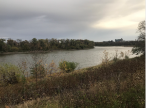
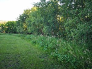
Border dividing the 2 areas of interest
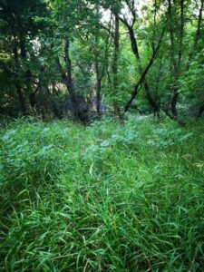
Forest Area

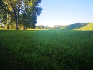
Hilly open grass area