Post 3: Ongoing Field Observations

Organism Studied: Alnus rubra (red alder)

Environmental Gradient: The environmental gradient of the study area is the rise in elevation from the shoreline to the railway and the corresponding changes in soil type, drainage and exposure to flood disturbance. Alnus rubra appears to dominate the lower elevations while coniferous species dominate the higher elevations.

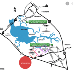
I have selected 4 sites along a 100 metre stretch of shoreline. Some parts of the shoreline are very steep and rocky, with limited vegetation. I consequently selected 4 sites that had a more gradual slope, and thus had sufficient vegetation to demonstrate a response to elevation, in regards to species type, abundance and maturity.
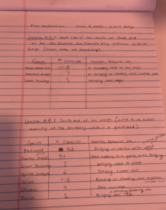
Site 1:
Roughly one quarter of the site is a low lying flat area, within 1 metre in vertical elevation from the waterline. The soil is soft, dense and deep, with a layer of leaf and stick detritus completely covering it. It appears that only species present here is alnus rubra, with many young plants covering the area as well as 5 mature trees over approximately 8 metres tall. There are two western red cedars and one western hemlock between 6 and 8 metres tall at the top of the slope, approximately 5 metres above the waterline.

Site 2:
Young alnus rubra plants are growing densely in the area below 2 metres in vertical elevation from the shoreline. The area has deep moist soil covered in leaf and stick matter. The slope rises steeply over large stone boulders. Above 2 metres in elevation, several mature western red cedars (6-12 metres) grow in loose sandy soil on the boulders. At around 5 metres in elevation, several Douglas firs and western red cedars (all over 5m tall), and some young western red cedars are present.

Site 3:
Site 3 rises and dips in several areas, and is mostly lower than 3 metres above the water level. The southern half of the site has a rocky surface with a thin layer of course soil that rises from the shoreline for 5 metres before sloping downwards to an area of thicker moist soils. The higher rocky ground has a several mature (5-15m tall) western red cedars and Douglas fir trees. The northern side of the site is lower lying, covered in grasses, mosses or dead leaf matter, with soft deep, moist soils. There are many smaller red alder plants and 5 mature red alder trees over 6 metres tall.

Site 4:
Most of site 4 is less than 1 metre above the lake water level. These areas have deep moist soils covered either by grasses or leaf detritus. There are many young alnus rubra growing in these low lying areas and 5 mature alnus rubra trees over 5 metres in height. At the top of the slope, approximately 5 metres above the water level are some young western red cedar trees.

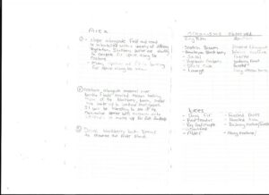
In all four sites the low-lying areas appear to be dominated by alnus rubra. These areas are mostly occupied by mosses, grasses and young alnus rubra, and the soils are deep, spongy and moist. The low areas are generally flat, and the land only rises where there are rock formations, which suggests to me that these areas are flood plains that have come about from erosion of softer parts of the shoreline. Walking further north along the shoreline I observed a grass and young red alder covered area beside a creek that was now submerged due to the increased creek flow from spring snow melts. This helped support my idea that these areas are likely subject to flood inundation. The vast majority of the alnus rubra in the low lying areas are young plants less than 50cm tall, which could be related to the frequency of flood disturbances, and red alder possibly being a colonizing species. The rocky, more elevated areas seemed to be dominated by mature conifers. Their age indicates that the area may not have not been subject to a significant flood disturbance for a long time, and the fact that there are no young conifer species at lower elevations might suggest that alnus rubra colonizes these areas before conifers do following floods, they out compete conifers there, or they are more resistant to flood disturbances so conifers are less likely to survive a flood.

I hence made the hypothesis that:
Alnus rubra will be the dominant tree species in flood prone areas of the Nita Lake shoreline.

Formal prediction:
Alnus rubra will be the most common tree species in areas of the riparian zone less than 2 metres in vertical elevation from the current waterline.

Predictor variable: elevation (continuous)

Response variable: abundance of tree species, age/size of trees (continuous)

Post 3: Ongoing Field Observations

The biological attributes that I intend to study are the species richness and abundance of forbs between the riparian, transitional, and upland zones of eastern bank of the South Saskatchewan River.

On June 13, 2020, I chose four locations adjacent to an overgrown pathway leading down, from the upland region (at the coordinates of 52.1384, -106.6400), towards the South Saskatchewan River. Based upon preliminary observations, each of the four locations (A, B, C, and D) (Fig. 1) have their own distinct vegetation structure. I have chosen to focus in on forb species because of the striking difference between species and abundance at each location. In addition, forbs appear to be present in each location; the same cannot be said for shrubs and trees (with shrubs occurring in high abundance in the upland and trees occurring in moderate abundance towards the river. Furthermore, based on these observations, species richness of forbs appears to be highest in the middle of the riparian zone, and lowest along the river and in the upland.

Therefore, I hypothesize that the distance between the river and the uplands influences the community structure of forb species. Along those lines, I predict that the richness and abundance of forbs will increase approaching the centre of the riparian zone. A potential response variable is the species richness and a potential explanatory variable is elevation. Both species richness and elevation are continuous variables.

Figure 1: The figure above is a drawing of the topography of the four sites (A, B, C, and D) that I have selected to observe the species richness and abundance of forbs.

Blog post 3: Ongoing Field Observation

Initially, while studying patterns in my chosen area along a riparian zone, tress had not leafed out yet, shrubs and flowers were also not in bloom. My notes consisted of observations on biodiversity (mostly avifauna), soil type and various ecotypes along the river. I noticed that ant hills were present throughout the area, but they were not consistent within each zone. At first, my observations did not show any patterns, but then more questioning on biotic and abiotic relationships further developed my research topic.

Upon further investigation, I have decided to study the presence/absence of ants in a riparian zone where vegetation, soil type and moisture changes throughout the elevation gradient situated on the north shore of the Highwood river.  The locations which I will continue to collect data from will include the river’s flood zone, a mixed grass plane with old cottonwood trees and a section of the south facing bank towards the uplands. While each location has a distinct landscape, I will also add a fourth section near vernal wetlands, located north-east from the river just below a steep bank, to add variety in soil type, moisture and vegetation cover.

Known species:

Western Thatcher Ant (Formica obscuripes) (see photo attached)

Hypothesis and prediction

Soil type, moisture and vegetation cover influences ant habitat preference. I predict that there will be more ant occurrences along an environmental gradient in concurrence with exposed, dryer and sandier soils.

Response variable: Ant presence/absence (categorical)

Predictor variables: Soil type (categorical), Soil moisture, vegetation cover (continuous)

Post 3: Ongoing Field Observations

With my next visit to Heritage Park I looked toward the stream located on the west side down from the gravel walking path. I’ve decided to study how the plant community changes along the riparian stream side as proximity to the stream changes. I want to know if these changes also occur with increasing changes in elevation.

I began my observations at the lowest point of the stream that I could access before there is a sudden drop into a ravine. Here the stream forms a small pond near a walking bridge. I took note of the vegetation in three rough points: near the stream, mid point up the bank and the upper portion of the bank near the gravel path.

I did the same at a second site near a bubbling pipe that allows water to flow through an area with a small dam, and then again once more further upstream.

My observations seem to indicate, for one, that the type of flora along the riparian bank seems to be more influenced by other factors than just the presence of the stream itself, but that there is a slight increase in plant diversity as proximity to the stream decreased. Some species known for their preference of moist soils such as salmon berry (Rubus Specabilis) were often present with few others such as fern species near the water, with the exception of the first site which also had some ground cover plants mixed in as well. Further back up the bank I found species such as black hawthorn (Crataegus douglasii) and other tree and shrub species mixed in with Himalayan blackberry (Rubus armeniacus) as well as other invasive species such as creeping buttercup (Rananculus repens). It seemed there was more diversity of species the farther away from the stream I observed. How far does this diversity go? Is there an average to the maximum amount of diversity before the level drops again?

Hypothesis – Proximity to the stream affects plant diversity at Heritage Park

Prediction – Plant diversity increases with an increase in elevation away from the stream. There is a maximum to this however before diversity averages, then drops.

Response variable – Number of plant species present (Continuous)

Explanatory variable – Distance from the stream (Continuous)


Post 3- Ongoing Field Observations

I am planning on studying the relationship between ungulate presence and the abundance of certain vegetation types. There are 3 zones of interest that I will observe: 80 year old Second growth Douglas Fir plantation, Riparian zone, and 18 year old harvested area. When walking through these areas I have noticed an abundance of Cervus canadensis roosevelti  sign in the riparian zone but none in the other areas, whereas I have noticed lots of Odocoileus hemionus columbianus sign in the harvested area but not as much in the forest and riparian zone. I have also observed a higher proportion of Vaccunium parvifolium and Gaultheria shallon in the forest than in either of the other two areas, whereas there is a higher abundance of Alnus rubra and other deciduous trees and shrubs in the riparian zone along with ground cover abundant in grasses. The harvested area is evenly covered in Vaccunium as well, but it seems to be less abundant than in the forest. Most of the ground cover in the harvested area at the moment is dead Pteridium aquilinum, but there are also new conifers as well as sparse large deciduous trees and shrubs.

Hypothesis: Cervus canadensis roosevelti sign is more abundant in areas with higher % cover of grasses and lower in areas with low % cover of grasses.

Prediction: Cervus canadensis roosevelti sign is more abundant in the Riparian zone where there is higher % cover of grasses and lower in the forest and harvested area where there is little to no grass cover.

Predictor variables: Riparian zone, Harvested area, Douglas Fir plantation (Categorical)

Response variables: % cover grasses (continuous), # of Cervus canadensis roosevelti scat groupings(Continuous)

Field Journal- scan0024

Blog Post 3 – Ongoing Field Observations

I plan on studying shorebird diversity at the Don Edwards San Francisco Bay National Wildlife Refuge. In particular, I plan on studying shorebird diversity attributes such as species richness, species abundance, species evenness, etc. in response to human presence. In order to study the response of shorebird diversity to human presence at this wildlife refuge, I chose three study locations with varying degrees of human presence across the marsh at the south end of the refuge. A map of the refuge with my chosen study locations are depicted in Figure 1. Location #1 is bordered by a highly urbanized environment, representing the peak of the gradient of human presence. Location #2 relatively closed off from human presence as it is bordered by a wet open grassland which is intersected by a road that leads to the wildlife refuge’s visitor center. This area does not house any trails or walkways and was chosen to represent a minimum of the human presence gradient. Location #3 borders the visiting center and houses walking trails, boarded pathways and bridges for visitors to explore the refuge, observe wildlife, etc.. I assumed that this location would represent an intermediate measure of human presence as this location only houses a visitor’s center and walking trails (minimal urbanization and much less human presence than the urban area bordering location #1). Figure 2 depicts my notes of observed shorebirds in the 3 study locations.

I hypothesize that one underlying process that may be influencing changes in shorebird diversity across a gradient of human presence (or nearby urbanization) may be an intolerance of the local refuge’s shorebird species to urban life or human presence.  Such intolerance may arise from habitat disturbance, pollution, noise, etc.. Based on this hypothesis, I predict that measures of shorebird diversity such as shorebird species richness, species evenness and species abundance should decrease with increases in human presence or urbanization. Specifically, Location #1 (nearby an urbanized environment) should have the least shorebird diversity and Location #2 (little to no human presence) should have the highest measures of shorebird diversity. Furthermore, Location #3 (containing walking trails and human visitors, with little urbanization) should have intermediate measures of shorebird diversity. Based on this hypothesis and predications, one potential response variable would be species richness (a measure of shorebird diversity) which would be a continuous variable. One potential explanatory variable would be the study location which corresponds to particular amount of human presence (Location #1 – high human presence, Location # 2 – little/no human presence, Location #3 – intermediate human presence), which would be a categorical variable.

Figure 1. Map of the Wildlife Refuge at the south end of the San Francisco Bay. The three study locations at which I studied shorebird diversity are depicted by squares (red being location #1, pink location #2 and purple being location #3).


Figure 2. Notes of shorebird observations at 3 study locations along the wildlife refuge south marsh.

Blog Post 3: Ongoing Field Observations

The biological attribute I have decided to study is the diversity of grasses in Wakamow Valley. I noticed that the preserved ecological zone of the valley had a wide variety of grasses compared to Conor Park and Tatawaw Park.

Wakamow Valley has quite a few distinct ecosystems/areas. The gradient I am using to observe in this project includes Tatawaw Park, an old wild animal park that was abandoned and closed down in the 80s. The old enclosures still stand with their concrete pads, and the old asphalt roads and parking lots are used for walking paths, frequented by bikers, hikers and their dogs. The second area is Conor Park, a well-maintained natural area often used for outdoor weddings, BBQ’s and walking. It also includes a large playground and parking area, but still has significant natural habitat intact. The third area of the gradient is the Kingsway Park Ecological Zone. This area is virtually untouched by humans anywhere other than the natural dirt walking path. The variation in grass diversity between these three distinct areas could be do to this gradient of increasing fragmentation. It could be that with increasing fragmentation, a decrease in biodiversity of grasses occurs. Based on this information, it can be assumed that Kingsway Park is the least fragmented area, Conor Park is moderately fragmented, and Tatawaw Park is significantly fragmented.

An alternative explanation is the heavy presence of uniform lawn grass in developed areas because of their anthropogenic selection for their aesthetic purposes and accessibility. To account for this possible confounding factor, clearly sodded areas should be excluded from the study.

Hypothesis: Grass biodiversity decreases with increased fragmentation of land.

Prediction: Fragmentation of habitat will negatively correlate with grass species diversity.

Response variable: diversity of grass species, continuous

Predictor variable: fragmentation level, continuous

Experimental design: regression

Blog Post 3 – Ongoing Field Observations

Blog Post 3 – 22-01-20

Upon examining the wooded area in the park closer on January 22nd at 1000 hours I have come to realize that selecting one biological attribute to study in the present winter conditions would be highly difficult considering the lack of vegetational growth. Therefore I have decided to study species diversity within Kinsmen park. The weather is at -6C and the sky is clear. Despite these warmer conditions, the area still appeared to lack any significant defining features. The biological attribute I have chosen to study is the density of White Birch (Betula papyrifera) compared to the density of Beaked Hazelnut (Coryluscornuta) in relation to location nearer or farther from the central pond.  After choosing these two subjects for comparison, I began looking at them across an environmental gradient on the northeastern side of the park where the vegetation was most dense. Five locations along this gradient were chosen, all approximately 15 feet apart

24-01-20

It is January 24th at 1200 hours. The skies are clear and the weather has warmed up a few degrees to -3C. There is a slight wind and it is very sunny outside. I examined the five locations along the gradient and noticed no observable changes in the trees and bush character. As trees are relatively slow growing, it is expected that there will be no changes in distribution or abundance for the tree species; however, changes in character for both species studied as the temperature continues to warm will be closely observed. 

26-01-20

It is January 26th at 1400 hours. The sky appears a bit overcast and the weather has dropped to -7C. There is no wind, but it is cold. In the White Birch area there are hare tracks and much of the snow on the trees has melted off. In other areas around the trees there appear to be much smaller tracks, perhaps those of a mouse. The hare and potential mouse tracks may suggest that as the temperature has warmed and snow has melted, the area is becoming more habitable for the animal life that is near the area. Surprisingly, I have noticed there to be more White Birch trees than I had originally estimated. They do not have any leaves, but their white and black, papery bark is easily distinguished even in the winter. The presence of the Beaked Hazelnut has been less prominent and leans further to the outermost edge of the gradient on the east side. 

29-01-20

It is January 29th at 1200 hours. The skies are clear and the weather is -2C. It is a relatively warm, sunny day. Along the gradient, the trees no longer have snow gathered on their branches. The same cannot be said for the bushes, which still hold snow in clumps at their base. Almost all of the vegetation in the park appears to be awaiting warmer temperatures to begin the regrowth process. I predict that White Birch will be seen in higher density closer to the pond while Beaked Hazelnut will be seen in higher density further away from the pond. I hypothesize that as the density of the White Birch increases, the density of the Beaked Hazelnut will decrease. I hypothesize this inverse relationship is due to the presence of moisture in the soil from the pond. One potential response variable from this is the density of trees versus shrubs measured in the number of trees or shrubs per square acre. This variable would be classified as categorical as the presence or absence of the two vegetation species are unique categories of measurement. One explanatory variable for these changes is the moisture content of the soil in the various locations of vegetation. This would be measured in g/m3 and is an example of a continuous variable as it can be measured on a continuous numerical scale. 


Field Journal – 1

Blog Post 3: Ongoing Field Observations


Over the past two weeks, I have been walking my field site wondering about what organism or environment I want to study. I have made several observations within my field journal, noting a wide range of possibilities, and have decided upon the Himalayan Blackberry (Rubus armeniacus) (HBB). This an invasive species to Vancouver Island that is found along the Wetland ecotone.

Vancouver Island is just coming into spring, and new growth is starting to occur within the ecosystem, but not on the blackberry vines yet. The first area I chose to observe was a slope alongside the road that quickly transitions of short grasses. The second area is at an area where high rivers and flooding have caused parts of the bank to erode, washing away parts of the transitional area containing blackberry bushes. It will be interesting to see if the blackberries colonize around the obstruction, or if native flora will be able to become established. The third area is a zone that borders woodland and my ecotone. The HBB becomes pervasive, walking through the ecotone becoming less developed with the existence of mature Cedars and Douglas Firs.

My Hypothesis: Himalayan Blackberry (Rubus Armeniacus) prefers a ecotone environment.

There is a visible transition zone from forest to wetlands along the ecotone with invasive species (Scotch Broom and Himalayan Blackberry), seemingly winning the race. Blackberry bushes seem to prefer the ecotone environment with minimal bushes appearing in forested areas. The categorical response variables could include recording the amount IN m^2 of HBB I observe in a perpendicular direction spanning into the ecotone. Predictor variables could be the amount of sunlight reaching the vine going into denser brush. An experimental design could include a one-way layout, by choosing patches of blackberry and documenting their health going into spring. I will choose ten replicates at a minimum making sure that each choice is independent of one another.

Blog Post 3: Ongoing Field Observation

Shannon Myles

February 3rd, 2020


By comparing the observations made on the field to the online plant database of the University of Texas (website: https://www.wildflower.org/), I was able to identify the four flowering plants of the site as the following: 

  1. Crotalaria Juncea L. or Sun hemp, the twolobed yellow flowers. 
  2. Helianthus debilis or Beach sunflower, the flowers with yellow petals and a black or yellow center of stamens.  
  3. Hepatica nobilis var. acuta sharp-lobed hepatica, the small white flowers with three-lobed green leaves. 
  4. Richardia brasiliensis small 6 petal purple flowers. They have long pointy green leaves. 

During my observations on the field, the concept of ecotone or transitional zone is what really hit me first. The abundance of flowers seemed to be proportional to the distance a certain patch of grass was from the beach. In other words, it seemed like the farther away I walked from the beach, the more flowers were scattered on the ground around me. It also seemed like the two types of yellow flowers were much less abundant all throughout the field. Though surprisingly, those bigger flowers appeared much closer to the beach than the majority of the smaller white or purple flowers.  

My hypothesis for this study will be that the natural step-cline creates a gradient in flower abundance that increases proportionally to its distance from the beachThe effect of the natural step-cline that is the beach, in this case, could be on nutrients in the soil or dryness of the soil. As observed, the soil in the area is very sandy, which is probably a result of its proximity to the beach. Very sandy and dry soil cannot support much plant life. Hence why the beach is one of the only places in the world where grass can not grow. So, my prediction for this research is that more flowers will appear as I walk away from the beach with my quadrat. No flowers should be observed in the first few meters from the beach as the soil will still be too dry and sandy. But, as I move towards the mainland, I predict that a few flowers will first appear and that abundance will increase after.  

The hypothesis I will test will be evaluated by the effect of the predictor variable (the distance of the quadrat from the beach) on the response variable (the abundance or number of flowers in the quadrat). By repeatedly gathering data on those two variables along the gradient, I’m hoping I will discover a trend in abundance variation. Considering that both the response and predictor variables will be continuous data, a regression design study will be used. 

Field Notes Blog Post 3