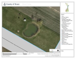
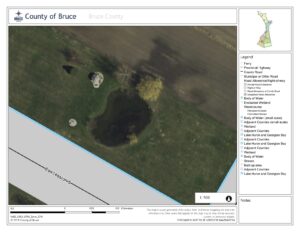
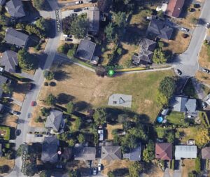
The main species in focus for my research will be Cattails and Lily Pads, and how they can become invasive to other species, as wells studying best practise pond management techniques. I am interested to see how the presence and density of either cattails or water Lillies or both effect the density of other species in the pond. In the past several years our pond has become extremely overgrown, the growth of new trees surrounding its perimeter. Alongside the massive increase in cattails and lillies. Below are air photos of the pond from 2010 (Figure 1) and 2015 (Figure 2). As you can see in just 5 years the amount of vegetation has doubled. To some property owners this may be an “eye sore,” however, my family does not mind. As the pond continues to evolve the amount of species that inhabit and utilize it as a resource have increased. The new trees surrounding the pond provide habitat for more bird species. As the weather continues to grow colder we will soon be having many Canadian Geese as visitors.
Figure 1: 2010 Air Photo of Pond
Figure 2: 2015 Air Photo of Pond
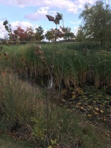
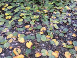
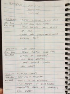
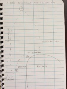
I am still brainstorming a concrete hypothesis but it will largely surround habitat space use from varying species in our pond and how the presence of one may effect another. Below are initial notes taken on October 4, 2019 along with photos of my study areas. (Figure 3- ). The graph in Figure 3 exemplifies a visual representation of the space utilized by varying factors in the pond, I will soon create a chart and more accurately record this data. Also note I am still working to identify two of the tree species. The drawing in Figure 4 represents how my study is going to be divided directionally, taking into account wind patterns, tree locations and how the pond is utilized by which species in each specific location.
The biological attribute I am planning to study in Cosens Bay in Kalamalka Lake Provincial Park is the distribution of common snowberry (Symphoricarpos albus), a deciduous shrub often densely colonial growing to approximately 0.5 – 3 m tall. Snowberry usually grows in mesic to dry meadows, disturbed areas, grasslands, shrublands and forests. Often scattered in coniferous forests and plentiful in broadleaved forests on water-shedding and water-receiving sites (E-Flora 2019). Snowberry is often associated with tall-Oregon grape (Mahonia aquifolium), birch-leaved spirea (Spiraea betulifolia) and rough goose neck moss (Rhytidiadelphus triquetrus) (E-Flora 2019).
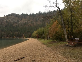
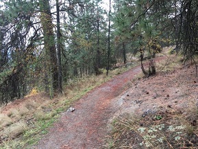
The three environmental gradients I am choosing to study in Cosens Bay include the riparian area of Kalamalka Lake, a transition zone between the riparian area and an upland area, and the upland area (Photo 1). Site 1 is the Riparian Area, Site 2 is the Transition Area and Site 3 is the Upland Area. On October 13, 2019 the three gradients were reviewed to observe the distribution, abundance and character of snowberry. On the day of the site visit, the temperature was approximately 7 degrees Celsius, cloudy with rain and observations were made between 9:00 am and 11:30 am.
Photo 1. View looking north illustrating three gradients from Riparian to Upland.
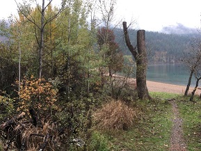
Site 1 (Riparian Area) is located approximately 10 m from Kalamalka Lake and snowberry is densely vegetated in shrub thickets along Cosens Bay Trail on the foreshore of Kalamalka Lake (Photo 2). The shrub appears relatively tall, with thick foliage with a large volume of berries. The leaves are bright green and the shrub appears to be thriving underneath a deciduous tree canopy of black cottonwood (Populus trichocarpa) and trembling aspen (Populus tremuloides) with dense shrub cover. The topography is relatively flat, facing south-west, with a wetland feature occurring upslope providing moist growing conditions.
Photo 2. View of the Riparian Area with dense snowberry under a deciduous canopy.
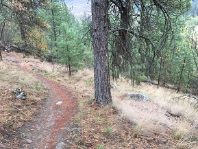
Site 2 (Transition Area) is located approximately 50 m upslope from Kalamalka Lake and snowberry is relatively sparse and appears shorter, with less foliage and less berry growth (Photo 3). The leaves are a lighter green and the shrubs were observed underneath a moderately dense canopy of ponderosa pine (Pinus ponderosa) trees. The topography is steeper than the Riparian Area and faces south east dominated by ponderosa pine and bluebunch wheatgrass (Pseudoroegneria spicata) with limited shrub coverage.
Photo 3. View of the Transition Area with sparse snowberry.
Site 3 (Upland Area) is located approximately 100 m upslope from Kalamalka Lake and snowberry is sparse to not present in this area (Photo 4). Shrubs that are present are small with less foliage and berry growth. The area is dominated by ponderosa pine, interior Douglas fir (Pseudotsuga menziesii), Saskatoon (Amelanchier alnifolia) and bluebunch wheatgrass. The tree canopy is open with little shrub cover. Other notable features in this area include relatively shallow soils with sporadic large boulders and the slope is steep, facing directly south.
Photo 4. View of the Upland Area with little to no snowberry present.
In summary, snowberry was observed in dense quantities in flat, moisture receiving areas (Riparian Area) and sparsely vegetated to not present in steeper, dry sloped areas (Transition Zone and Upland Area).
The underlying processes that are may be contributing to the distribution and abundance of snowberry includes the hydrological cycle and moisture availability in soils. Based on my observations and the concept of limiting physical factors, water retention in the soil may be limiting snowberry to moisture receiving environments which is indicative of relatively flat topography.
One hypothesis to prove or disprove my observation is, “The distribution of common snowberry is determined by slope”. My prediction is “Common snowberry will be present in areas where slope is less than 20% grade”.
My experimental design would aim to empirically validate the pattern, that common snowberry distribution is limited to areas with less than 20% grade or that common snowberry distribution diminishes as percentage slope increases.
Based on my hypothesis that “The distribution of common snowberry is determined by slope”, one response variable could be the presence or absence of common snowberry which would be categorical. One explanatory/predictor variable could be the percentage slope, which would be continuous. Based on a categorical response variable and a continuous explanatory/predicator variable a logistic regression design could be utilised.
References:
E-Flora BC Electronic Atlas of the Flora of British Columbia [Internet]. 2019. Lab for Advanced Spatial Analysis, Department of Geography, University of British Columbia [cited October 14, 2019]. Available from: https://ibis.geog.ubc.ca/biodiversity/eflora/
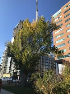
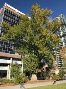
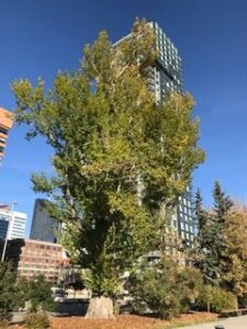
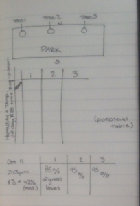
I revisited the park Oct 11, 2019 at 2:13pm. The temperature was 6°C and humidity at 42%. From my previous observations, the trees looked different in all areas of the park, some were decaying while others are still mostly green. Hence, I have chosen the study how the temperature, and especially the humidity from changes in weather, are going to affect the changes in certain trees. there are three deciduous trees, comparable in size and all quite bigger than the other trees, all located along the North side of the park.
Hypothesis: The colder and dryer the weather gets over the course of Autumn, the more the leaves of the trees will change.
Prediction: As the weather gets colder and dryer, then all the leaves in each of the three trees should change at approximately the same rate.
Response Variable: Amount of color change in leaves in each tree. It will be a continuous variable as the amount of color changed leaves from green to yellow is a % of all the leaves on the tree.
Explanatory Variable: Level of humidity. It is a categorical variable as humidity will be placed in low (< 30%), medium (30-70 %), and high (>70%) levels.
I plan to study lichen growth on tree bark in Stanley Park. In the field, I chose to observe a line of 10 trees (approx. 75 m in length, North to South) in an immature stand (30 – 99 years) that ran from north to south. The environmental gradient spanned multiple locations that varied by canopy coverage and sunlight penetration. I recorded observations for each tree, which included my best in-field description of the tree genus (spruce, fir, cedar, beech). What was classified as spruce in the field, was determined to be hemlock. I recorded the approximate percent coverage of lichen, from eye-level to the base of the tree trunk. I recorded the side of the tree (ie. north, south, east, or west) with the predominant lichen coverage. I scored each tree trunk for light penetration based on canopy coverage and forest density, which I estimated in the field. The following described how each tree was scored for approximate sunlight penetration in the forested area:
0 – Full canopy coverage, dense forest; no light penetration to tree base/trunk
1 – Some openings in canopy, dense forest; minimal light penetration to tree base/trunk
2 – Medium openings in canopy coverage; forested area; visible light penetration to tree base/trunk
3 – No canopy coverage, wide open area; full visible light penetration to tree base/trunk for most of the day
Moss and or lichen coverage was visually estimated from eye level to the base of the tree. Moss/lichen percent (%) coverage was approximated using the following score system:
0 – Little to no visible lichen coverage (i.e. 0 – 10% coverage from eye level to base of tree)
1 – Minimal, patchy lichen coverage (i.e. 10 – 30% coverage from eye level to base of tree)
2 – Medium lichen coverage (i.e. 30 – 70% coverage from eye level to base of tree)
3 – High lichen coverage (i.e. 70 – 100%).
Photo 1. Field Observations for lichen/moss coverage and tree speciesPhoto 2. Rough ideas on how to score light penetration/canopy coverage and lichen/moss growthPhoto 3. 10th tree sampled and concluding field notesPhoto 4. One of six fir or hemlock trees examined for lichen growth
Summary of Observations:
Estimating sunlight penetration based on canopy coverage was difficult to quantify, and would present a challenge to accurately measure in the field without proper instrumentation. Overall, 6 of 6 fir/hemlock trees had some degree of lichen coverage. When compared to beech, only 1 of 3 had observable lichen growth. No lichen growth was observed on the 1 cedar observed. One notable difference between these three tree types is the visible rugosity, texture, and thickness of their bark. The fir and hemlock trees had thick, textured bark. In contrast, the beech and cedar bark was noticeably more sooth, with less cracks and crevasses. In summary, I have chosen a hypothesis that applies to one point on the gradient, specifically an area of trees that experience the same exposure to sunlight.
Hypothesis:
Fir and hemlock tree bark provides more suitable growth substrate for lichen in Stanley park.
Prediction:
Lichen growth is more common on bark of fir and hemlock trees, compared to beech and cedar bark in Stanley Park.
The presence or absence of lichen is a response variable, that could be treated as a categorical variable (i.e. yes or no) or a continuous variable (i.e. if yes = 1, and no = 0). A predictor variable could be the tree genus (categorical).
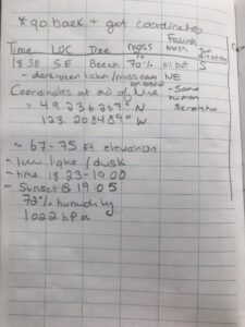
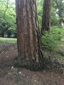
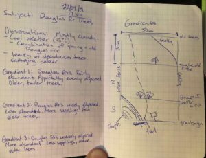
I plan to study the Douglas Fir trees found at the junction of Johnny’s trail and Douglas Fir trail in Canmore, AB.
Notable locations along the environmental gradient of my location include: a flat, open forested area; a more densely forested area on a slope; and a rocky, sparsely vegetated spring run-off gully.
The first location has a variety of shrubbery, clover, and rose bushes; along with randomly dispersed Douglas fir trees in low abundance. The trees appear to grow as individuals. On average, there appears to be more Douglas fir saplings in comparison to older trees. All Douglas fir trees present appear to have branches evenly dispersed around the tree’s radius.
The second location has less of a variety of shrubbery, clover, and rose bushes. There are more densely dispersed Douglas fir trees in great abundance. The trees appear to grow in clumps. There appear to be more older trees than saplings.
The third location has very few plants. There are a few immature Douglas fir trees growing around the edges of the gully, along with a few shrubs. The Douglas fir trees grow alone and are nearly all older trees. The trees are widely dispersed and in low abundance.
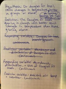
My hypothesis I wish to test is as follows: do Douglas fir trees better resist cooling temperatures of changing seasons in groups or as individuals? I predict that the trees will fair better against the temperature change in groups.
A possible responding variable is the abundance, distribution, and size of the Douglas fir trees in each location. This variable is continuous. A possible predictor variable is the ambient air temperature and weather. This variable is also continuous.
I will be looking at the weather and the number of bees that visit the plants within the bee garden. Does the temperature seem to affect the number of bees? Or does the weather?
My response variable is the number of bees. My predictor variable is the weather. I believe these variables would be continuous because it is an infinite number between these two variables.
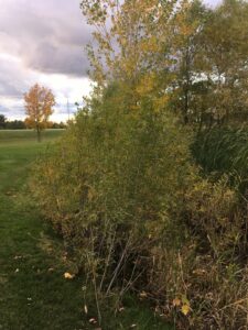
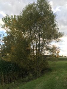
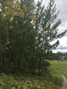
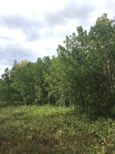
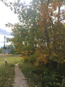
Aspen trees at bottom of hill, looking EastAspen trees on middle of hill, looking WestAspen trees at top of hill, looking East
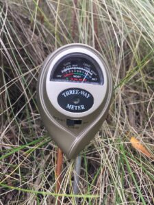
The purpose of this fieldwork was to observe aspen trees, Populus tremuloides, located in Whispering Woods. One of the environmental gradients present at this location is a 12m change in elevation from the bottom to the top of the Woods. Therefore, I chose to observe health attributes of P. tremuloides trees located at the bottom, middle, and top of this hill. The specific attributes I observed were leaf colour (percent of primarily yellow leaves on the trees), soil moisture (measured using a HoldAll® Moisture, Light, and pH Meter™), and soil pH (also measured using a HoldAll® Moisture, Light, and pH Meter™). Soil moisture and pH measures were taken 20-30cm from the base of the tree. Additionally, I looked at general differences in the distribution, abundance, and character of these trees located at the bottom, middle, and top of the hill.
HoldAll® Moisture, Light, and pH Meter™ reading moisture level of soil near a tree at the bottom of the hillObservations recorded in field journal describing differences in leaf colour percentage, average soil moisture levels, average pH levels, and density of trees located along the gradient of the hill slope.Observations from field journal measuring the soil moisture level and pH of n=10 trees chosen using convenience sampling for the bottom, middle, and top of the hill. Average soil moisture and pH also calculated, with rankings shown.
As indicated from the field journal documentation, there were character differences present including the percentage of yellow leaves, soil moisture, and soil pH of the 30 trees sampled (10 from each level of gradient). The bottom of the hill contained trees with almost completely green leaves, a higher average moisture, and a medium average pH. The top of the hill contained trees with primarily green leaves on its West side, and primarily yellow leaves on its East side. Further, trees on the top had the lowest average soil moisture, and most alkaline average soil pH. Trees located in the middle of the hill had a combination of characteristics from both.
Additionally, I observed differences in the abundance of trees, as the top NW contained the densest area of trees, while the bottom SE corner contained the least. These dense trees were also smaller in size on average. The distribution of yellow coloured leaves also was a clear finding, with primarily yellow-leaved trees located on the East side, and primarily green-leaved trees located on the West side for both the trees sampled from the middle and top of the hill. Another important note is that there were not enough trees to sample from the bottom SE corner relative to the width of the hill, so samples taken from the bottom of the hill were taken from trees all on the SW side.
From these observations, I have compiled a hypothesis and a prediction. It is important to note that in this stage of my Field Project, I am choosing to define the “health” of these trees as green leaves, high soil moisture, and a neutral soil pH. As the Fall season progresses, I hope to include other relevant indicators, such as rate of leaf loss, and perhaps water infiltration rate.
My hypothesis is that there is a significant difference in P. tremuloides health (based on the definition above) among trees located along the elevation gradient of Whispering Woods hill. My null hypothesis would therefore be that there is no difference in P. tremuloides health among trees located along the elevation gradient of Whispering Woods hill; any difference is due to chance alone.
Based on this hypothesis, I can make certain predictions regarding the attributes of health I have chosen. I predict that trees located at the bottom of the hill will have a better overall health, indicated by a higher average green leaf percentage, higher soil moisture, and a neutral soil pH. Conversely, I predict that trees located at the top of the hill, on average, will have a worse overall health, indicated by a lower green leaf percentage, lower soil moisture, and a more alkaline soil pH. These predictions are based on my previous knowledge of what plants require to grow optimally.
From these predictions, the response variable would be indicators of tree health (soil moisture, percent green leaves, soil pH) which is a continuous variable. The explanatory variable would be the position of the tree on the hill (bottom or top) which is a categorical variable.
The organism that I have chosen to study is the perennial plant Canada goldenrod (Solidago canadensis). As mentioned in a previous post, I observed that the height and density of this plant varied depending on its location. In some areas the plants were completely in the shade, while in other areas they were exposed to direct sunlight. Therefore, the environmental gradient I have chosen is the degree of sunlight exposure. The three locations along the environmental gradient I have identified are areas where the goldenrod has access to direct sunlight, has only partial sunlight exposure, and is completely in the shade. I have labelled these areas as high, moderate, and low levels of sunlight exposure, respectively. In the areas of low sun exposure, the plants had the lowest density, appeared to be the shortest, had minimal flowering buds, and were sparsely distributed. In the areas of moderate sun exposure, the plants appeared to be slightly taller than the plants in the low sun exposure area and had greater plant density. In the areas of high sun exposure, the plants were the tallest, appeared to have the greatest density, and a majority of the goldenrod plants exhibited flowering buds.
Hypothesis: Level of sunlight exposure affects the growth of Canada goldenrod (Solidago canadensis).
Prediction: If this hypothesis is true, then it is predicted that the height of Canada goldenrod will increase with the level of sunlight exposure.
Response variable: Plant height. This is a continuous variable as it is measured on a numerical scale in inches.
Prediction (explanatory) variable: Level of sunlight exposure. This is a categorical variable as we are observing, not measuring, the categories low, moderate, and high sunlight exposure.
I revisited my chosen area on August 4th 2019 at 13:37. I have decided to conduct my field research study on the plant species Trifolium repens (common name White Clover). Specifically, the distribution and abundance of Trifolium repens across the three locations I identified along the environmental gradient.
Trifolium repens is a small plant which appears to mainly grow in clusters. Most often they are found to have three balloon shaped leaves which are approximately 0.5 – 1 cm long and their stem is approximately 1-3 cm long.
The 3 locations I chose each differed in the amount of shade/coverage that was provided to the clovers. The 3 locations were as follows; shade, no shade and partial shade. The clovers did grow in each of the three locations, however there was a distinct difference in the abundance of clovers across the locations. The “no shade” location appeared to have the highest abundance of clovers, the “shade” location had the lowest abundance and the “partial shade” area was in between.
Furthermore, in the “partial shade” location I noticed that the phenotypic expression of the clovers differed. The clovers I studied in that location had much larger leaves, approximately 5mm longer than the leaves found on clovers in other areas. At a far glance it appeared that the abundance was highest in this location, however with closer inspection I noted that apparent abundance was most likely due to the larger clovers.
Hypothesis : Plants need sufficient access to many natural resources, including sunlight. With lack of sunlight the plants cannot thrive.
My prediction is that Trifolium repens will grow in higher abundance in sunlight, therefore the abundance will be highest in the “no shade” location.
One potential response variable is the abundance of Trifolium repens (continuous). One potential predictor variable is the amount of access Trifolium repens has to sunlight (categorical).
Based on the experimental design tutorial I deduced that my experimental design would be classified as ANOVA
I have decided to do my research field study on the plant species Hydrocotyle heteromeria (Wax weed or Pennywort). I found it in a large patch around a wet soil area, underneath the mature Pyrus communis (pear tree). There were only a few areas I spotted with Waxweed species in large quantities, but perhaps with the field research project I may find smaller patches within the grassy areas. After I had completed a Tru.ca Library and internet research, it sounds as if the plant species prefers moist areas and grows in areas of yards, golf greens or forests that do not have well drained soil.
I found that by documenting the observable gradient of the landscape (attached photos), the plant species is clustered around areas 1 and 2. Both of the first two selected sites are in areas of lower soil levels. I notice that in area 1, where I first noticed the large clusters of Pennywort, there are small pockets of even lower soil levels around the base of the Pyrus tree. The Hydrocotyle heteromeria is found in large abundance in these pockets. In observation region 2, there is still large amounts of the plant found, but it looks as though there is a decreased amount of large clusters. It seems as though the plants are clustered around the base of the tree. There could possibility be a symbiotic relationship with the tree or the plant may prefer nutrients received closer to the mature tree. The nutrient level in the center and drier area of the landscape may differ from the nutrient level near the tree, especially because there are many large trees on the non-study side of the fence (approximately 4 feet from the location of found Waxweed). In both observational regions 3 and 4, there was no sign of the species, so distribution and abundance has decreased drastically.
I believe that these pockets of lower soils levels catch and contain more water. There would be an abundance of water especially around the base of the tree as the area receives less sunlight, and the lower soils levels would accumulate more water. There would also be an accumulation of water in areas 1 and 2 because of the winter water run-off from the tree.
Hypothesis: The distribution of Hydrocotyle heteromeria in the Christchurch New Zealand backyard landscape is limited to areas of soil with high moisture content. My
Prediction: H. heteromeria is seen in areas of high moisture and the plants abundance decreases at the soil becomes increasing dry.
Prediction Variable: Soil moisture. High moisture content or Low moisture content is a Categorical Variable.
Response Variable: Plant numbers decrease as soils moisture decreases. The sample units would be Categorical as “absent or present.”