Between March 17 and June 2, 2019, I made 9 visits to my study area, totaling 14.75 hours of field observation and 188 data points with associated covariates; 159 of which were indicative of terrestrial vertebrates. Where possible, photographs of wildlife or indicators of their presence were taken and stamped with UTM locations, or identified visually or by song. I was using a cell phone camera and am a poor photographer so frequently I was unable to capture images of animals I observed. I decided to end my investigations on June 2, given that a significant increase in observed industrial (e.g., water withdrawal and nearby industrial noise, scheduled changes to river flow regime), recreational (e.g., human presence and deposition of wildlife attractants) and transit activity (e.g., off-road vehicles, boating) which had the potential to affect wildlife activity in the direct vicinity of my study area. This seemed a reasonable if not necessary place to end my field observations.
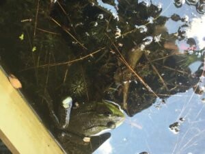
As I collected data over time (e.g., prior do, during and after spring freshet), the edges of the floodplain and riparian areas became clearly defined and the terrestrial vertebrate community structure within each emerged as evidenced by sightings, audible calls, observations of tracks, animal sign as well as active nests, dams and dens. Despite the changing seasonal conditions, habitat use by certain species and classes of vertebrates remained relatively consistent in the riparian area and floodplain as well as in and above the open water. For example, Tundra Swans were only observed in open-water on the Halfway River while Geese were observed everywhere but open-water on the Halfway river (i.e., floodplain, riparian area and open-water on the Peace River); dabbling ducks were only observed on open-water in the Peace River. Western Toad tadpoles were only observed in pools on the floodplain while both grouse species I observed were in the riparian area. All of the carnivorous species I observed were on the floodplain.
Given that my study location is at the confluence of a regulated and a non-regulated river, the Peace River and Halfway Rivers respectively, I was presented with a unique opportunity to examine how regulation of river level and discharge could be related to vertebrate habitat use and community structure. Both rivers are influenced similarly at the confluence by local snow and ice melt, but only the Peace River is regulated by upstream hydroelectric infrastructure. The area most affected by rising water level and flow rate or discharge is the floodplain, given large areas of it are inundated daily due to fluctuating river level.
Thus, the biological attribute I am interested in examining is vertebrate community structure in discrete areas (i.e., riparian, floodplain, and open-water areas) at the confluence of the Peace and Halfway Rivers.
My hypothesis is that short-term fluctuations in river level and/or discharge affect terrestrial vertebrate habitat use, and thus the community structure of riparian, floodplain and open-water areas of the Peace and Halfway Rivers deferentially.
If the community structure of terrestrial vertebrates is affected by short term fluctuations in river level and discharge, I predict that the species richness and diversity of the floodplain will fluctuate to a greater degree than the riparian and open-water areas relative to hydro metric conditions.
Response Variable: Species diversity; continuous
Explanatory Variable I: River level; continuous
Explanatory Variable II: Area; categorical
Note: UTM extraction is proving to take much longer than I had anticipated and will be included at a later time for anyone interested!
| Date |
Time |
Time Spent |
Area |
UTM |
Temperature |
Precipitation |
Wind |
Species |
Observation |
Approximate Halfway Level |
Approximate Halfway Discharge |
Approximate Peace Level |
Approximate Peace Discharge |
| 03/17/09 |
12:00-15:30 |
3.5 h |
Riparian |
|
6C |
None |
Light; west |
Bald Eagle |
Nest |
0.760 m |
19.0 m3/s |
2.56 m |
860 m3/s |
| 03/17/09 |
12:00-15:30 |
3.5 h |
Riparian |
|
6C |
None |
Light; west |
Bank Swallow |
Nest |
0.760 m |
19.0 m3/s |
2.56 m |
860 m3/s |
| 03/17/09 |
12:00-15:30 |
3.5 h |
Floodplain |
|
6C |
None |
Light; west |
Canada Goose |
Scat |
0.760 m |
19.0 m3/s |
2.56 m |
860 m3/s |
| 03/17/09 |
12:00-15:30 |
3.5 h |
Floodplain |
|
6C |
None |
Light; west |
Canada Goose |
Visual |
0.760 m |
19.0 m3/s |
2.56 m |
860 m3/s |
| 03/17/09 |
12:00-15:30 |
3.5 h |
Peace |
|
6C |
None |
Light; west |
Canada Goose |
Visual |
0.760 m |
19.0 m3/s |
2.56 m |
860 m3/s |
| 03/17/09 |
12:00-15:30 |
3.5 h |
Overhead |
|
6C |
None |
Light; west |
Common Raven |
Visual |
0.760 m |
19.0 m3/s |
2.56 m |
860 m3/s |
| 03/17/09 |
12:00-15:30 |
3.5 h |
Floodplain |
|
6C |
None |
Light; west |
Coyote |
Tracks |
0.760 m |
19.0 m3/s |
2.56 m |
860 m3/s |
| 03/17/09 |
12:00-15:30 |
3.5 h |
Floodplain |
|
6C |
None |
Light; west |
Moose |
Scat |
0.760 m |
19.0 m3/s |
2.56 m |
860 m3/s |
| 03/17/09 |
12:00-15:30 |
3.5 h |
Riparian |
|
6C |
None |
Light; west |
Mule Deer |
Visual |
0.760 m |
19.0 m3/s |
2.56 m |
860 m3/s |
| 03/17/09 |
12:00-15:30 |
3.5 h |
Floodplain |
|
6C |
None |
Light; west |
Mule Deer |
Scat |
0.760 m |
19.0 m3/s |
2.56 m |
860 m3/s |
| 03/17/09 |
12:00-15:30 |
3.5 h |
Riparian |
|
6C |
None |
Light; west |
Sharp-tail Grouse |
Visual |
0.760 m |
19.0 m3/s |
2.56 m |
860 m3/s |
| 03/17/09 |
12:00-15:30 |
3.5 h |
Floodplain |
|
6C |
None |
Light; west |
Unknown Dabbling Duck Breeding Pair |
Visual |
0.760 m |
19.0 m3/s |
2.56 m |
860 m3/s |
| 03/24/19 |
13:00-4:30 |
1.5 h |
Floodplain |
|
11C |
None |
Light; west |
Canada Goose |
Scat |
0.795 m |
21.0 m3/s |
2.49 m |
800 m3/s |
| 03/24/19 |
13:00-4:30 |
1.5 h |
Floodplain |
|
11C |
None |
Light; west |
Canada Goose |
Tracks |
0.795 m |
21.0 m3/s |
2.49 m |
800 m3/s |
| 03/24/19 |
13:00-4:30 |
1.5 h |
Overhead |
|
11C |
None |
Light; west |
Canada Goose |
Visual |
0.795 m |
21.0 m3/s |
2.49 m |
800 m3/s |
| 03/24/19 |
13:00-4:30 |
1.5 h |
Peace |
|
11C |
None |
Light; west |
Canada Goose |
Visual |
0.795 m |
21.0 m3/s |
2.49 m |
800 m3/s |
| 03/24/19 |
13:00-4:30 |
1.5 h |
Floodplain |
|
11C |
None |
Light; west |
Common Raven |
Tracks |
0.795 m |
21.0 m3/s |
2.49 m |
800 m3/s |
| 03/24/19 |
13:00-4:30 |
1.5 h |
Overhead |
|
11C |
None |
Light; west |
Common Raven |
Visual |
0.795 m |
21.0 m3/s |
2.49 m |
800 m3/s |
| 03/24/19 |
13:00-4:30 |
1.5 h |
Floodplain |
|
11C |
None |
Light; west |
Coyote |
Tracks |
0.795 m |
21.0 m3/s |
2.49 m |
800 m3/s |
| 03/24/19 |
13:00-4:30 |
1.5 h |
Riparian |
|
11C |
None |
Light; west |
Elk |
Tracks |
0.795 m |
21.0 m3/s |
2.49 m |
800 m3/s |
| 03/24/19 |
13:00-4:30 |
1.5 h |
Floodplain |
|
11C |
None |
Light; west |
Mouse |
Tracks |
0.795 m |
21.0 m3/s |
2.49 m |
800 m3/s |
| 03/24/19 |
13:00-4:30 |
1.5 h |
Floodplain |
|
11C |
None |
Light; west |
Mule Deer |
Scat |
0.795 m |
21.0 m3/s |
2.49 m |
800 m3/s |
| 03/24/19 |
13:00-4:30 |
1.5 h |
Floodplain |
|
11C |
None |
Light; west |
Mule Deer |
Tracks |
0.795 m |
21.0 m3/s |
2.49 m |
800 m3/s |
| 03/24/19 |
13:00-4:30 |
1.5 h |
Riparian |
|
11C |
None |
Light; west |
Mule Deer |
Scat |
0.795 m |
21.0 m3/s |
2.49 m |
800 m3/s |
| 03/24/19 |
13:00-4:30 |
1.5 h |
Peace |
|
11C |
None |
Light; west |
Tundra Swans |
Visual |
0.795 m |
21.0 m3/s |
2.49 m |
800 m3/s |
| 03/24/19 |
13:00-4:30 |
1.5 h |
Floodplain |
|
11C |
None |
Light; west |
Wolf |
Tracks |
0.795 m |
21.0 m3/s |
2.49 m |
800 m3/s |
| 03/31/19 |
12:30-14:30 |
2.0 h |
Floodplain |
|
5C |
Light; rain |
Light; west |
Bald Eagle |
Visual |
0.900 m |
100.0 m3/s |
2.49 m |
890 m3/s |
| 03/31/19 |
12:30-14:30 |
2.0 h |
Peace |
|
5C |
Light; rain |
Light; west |
Canada Goose |
Visual |
0.900 m |
100.0 m3/s |
2.49 m |
890 m3/s |
| 03/31/19 |
12:30-14:30 |
2.0 h |
Overhead |
|
5C |
Light; rain |
Light; west |
Common Raven |
Visual |
0.900 m |
100.0 m3/s |
2.49 m |
890 m3/s |
| 03/31/19 |
12:30-14:30 |
2.0 h |
Floodplain |
|
5C |
Light; rain |
Light; west |
Coyote |
Tracks |
0.900 m |
100.0 m3/s |
2.49 m |
890 m3/s |
| 03/31/19 |
12:30-14:30 |
2.0 h |
Floodplain |
|
5C |
Light; rain |
Light; west |
Mule Deer |
Scat |
0.900 m |
100.0 m3/s |
2.49 m |
890 m3/s |
| 03/31/19 |
12:30-14:30 |
2.0 h |
Riparian |
|
5C |
Light; rain |
Light; west |
Mule Deer |
Scat |
0.900 m |
100.0 m3/s |
2.49 m |
890 m3/s |
| 03/31/19 |
12:30-14:30 |
2.0 h |
Riparian |
|
5C |
Light; rain |
Light; west |
Rabbit |
Visual |
0.900 m |
100.0 m3/s |
2.49 m |
890 m3/s |
| 04/15/19 |
13:00-14:30 |
1.5 h |
Floodplain |
|
8C |
Light; rain – Clearing |
Light; west |
Beaver |
Chewed trees |
0.87 m |
90.0 m3/s |
2.37 m |
650 m3/3 |
| 04/15/19 |
13:00-14:30 |
1.5 h |
Floodplain |
|
8C |
Light; rain – Clearing |
Light; west |
Beaver |
Visual |
0.87 m |
90.0 m3/s |
2.37 m |
650 m3/3 |
| 04/15/19 |
13:00-14:30 |
1.5 h |
Floodplain |
|
8C |
Light; rain – Clearing |
Light; west |
Canada Goose |
Visual |
0.87 m |
90.0 m3/s |
2.37 m |
650 m3/3 |
| 04/15/19 |
13:00-14:30 |
1.5 h |
Peace |
|
8C |
Light; rain – Clearing |
Light; west |
Canada Goose |
Visual |
0.87 m |
90.0 m3/s |
2.37 m |
650 m3/3 |
| 04/15/19 |
13:00-14:30 |
1.5 h |
Overhead |
|
8C |
Light; rain – Clearing |
Light; west |
Canada Goose |
Visual |
0.87 m |
90.0 m3/s |
2.37 m |
650 m3/3 |
| 04/15/19 |
13:00-14:30 |
1.5 h |
Riparian |
|
8C |
Light; rain – Clearing |
Light; west |
Chickadee |
Singing |
0.87 m |
90.0 m3/s |
2.37 m |
650 m3/3 |
| 04/15/19 |
13:00-14:30 |
1.5 h |
Overhead |
|
8C |
Light; rain – Clearing |
Light; west |
Common Raven |
Visual |
0.87 m |
90.0 m3/s |
2.37 m |
650 m3/3 |
| 04/15/19 |
13:00-14:30 |
1.5 h |
Floodplain |
|
8C |
Light; rain – Clearing |
Light; west |
Coyote |
Scat |
0.87 m |
90.0 m3/s |
2.37 m |
650 m3/3 |
| 04/15/19 |
13:00-14:30 |
1.5 h |
Floodplain |
|
8C |
Light; rain – Clearing |
Light; west |
Coyote |
Tracks |
0.87 m |
90.0 m3/s |
2.37 m |
650 m3/3 |
| 04/15/19 |
13:00-14:30 |
1.5 h |
Floodplain |
|
8C |
Light; rain – Clearing |
Light; west |
Muskrat |
Visual |
0.87 m |
90.0 m3/s |
2.37 m |
650 m3/3 |
| 04/15/19 |
13:00-14:30 |
1.5 h |
Riparian |
|
8C |
Light; rain – Clearing |
Light; west |
Ruffed Grouse |
Drumming |
0.87 m |
90.0 m3/s |
2.37 m |
650 m3/3 |
| 04/15/19 |
13:00-14:30 |
1.5 h |
Riparian |
|
8C |
Light; rain – Clearing |
Light; west |
Unknown Mammal |
Den |
0.87 m |
90.0 m3/s |
2.37 m |
650 m3/3 |
| 04/15/19 |
13:00-14:30 |
1.5 h |
Riparian |
|
8C |
Light; rain – Clearing |
Light; west |
Unknown Wood Pecker |
Drumming |
0.87 m |
90.0 m3/s |
2.37 m |
650 m3/3 |
| 04/21/19 |
13:45-15:15 |
1.5 h |
Floodplain |
|
11.5 |
None |
Moderate; West |
Canada Goose |
Tracks |
1.19 m |
140 m3/s |
2.33 m |
625 m3/s |
| 04/21/19 |
13:45-15:15 |
1.5 h |
Peace |
|
11.5 |
None |
Moderate; West |
Canada Goose |
Visual |
1.19 m |
140 m3/s |
2.33 m |
625 m3/s |
| 04/21/19 |
13:45-15:15 |
1.5 h |
Overhead |
|
11.5 |
None |
Moderate; West |
Common Raven |
Visual |
1.19 m |
140 m3/s |
2.33 m |
625 m3/s |
| 04/21/19 |
13:45-15:15 |
1.5 h |
Floodplain |
|
11.5 |
None |
Moderate; West |
Coyote |
Scat |
1.19 m |
140 m3/s |
2.33 m |
625 m3/s |
| 04/21/19 |
13:45-15:15 |
1.5 h |
Floodplain |
|
11.5 |
None |
Moderate; West |
Coyote |
Tracks |
1.19 m |
140 m3/s |
2.33 m |
625 m3/s |
| 04/21/19 |
13:45-15:15 |
1.5 h |
Peace |
|
11.5 |
None |
Moderate; West |
Mallard (breeding pair) |
Visual |
1.19 m |
140 m3/s |
2.33 m |
625 m3/s |
| 04/21/19 |
13:45-15:15 |
1.5 h |
Floodplain |
|
11.5 |
None |
Moderate; West |
Moose |
Tracks |
1.19 m |
140 m3/s |
2.33 m |
625 m3/s |
| 04/21/19 |
13:45-15:15 |
1.5 h |
Floodplain |
|
11.5 |
None |
Moderate; West |
Mule Deer |
Tracks |
1.19 m |
140 m3/s |
2.33 m |
625 m3/s |
| 04/21/19 |
13:45-15:15 |
1.5 h |
Floodplain |
|
11.5 |
None |
Moderate; West |
Mule Deer |
Tracks |
1.19 m |
140 m3/s |
2.33 m |
625 m3/s |
| 04/21/19 |
13:45-15:15 |
1.5 h |
Floodplain |
|
11.5 |
None |
Moderate; West |
Unknown Carnivore |
Scat |
1.19 m |
140 m3/s |
2.33 m |
625 m3/s |
| 4/21/19 |
13:45-15:15 |
1.5 h |
Riparian |
|
11.5 |
None |
Moderate; West |
Bald Eagle |
Visual |
1.19 m |
140 m3/s |
2.33 m |
625 m3/s |
| 4/21/19 |
13:45-15:15 |
1.5 h |
Floodplain |
|
11.5 |
None |
Moderate; West |
Squirrel |
Visual |
1.19 m |
140 m3/s |
2.33 m |
625 m3/s |
| 4/21/19 |
13:45-15:15 |
1.5 h |
Floodplain |
|
11.5 |
None |
Moderate; West |
Unknown Sparrow |
Visual |
1.19 m |
140 m3/s |
2.33 m |
625 m3/s |
| 4/21/19 |
13:45-15:15 |
1.5 h |
Riparian |
|
11.5 |
None |
Moderate; West |
Unknown Sparrow |
Nest |
1.19 m |
140 m3/s |
2.33 m |
625 m3/s |
| 4/29/19 |
15:48-17:45 |
2.0 h |
Riparian |
|
8.5 |
rain; clear; snow |
Light; west |
Blue Jay |
Visual |
1.01 m |
110 m3/s |
2.26 |
600 m3/s |
| 4/29/19 |
15:48-17:45 |
2.0 h |
Floodplain |
|
8.5 |
rain; clear; snow |
Light; west |
Canada Goose |
Scat |
1.01 m |
110 m3/s |
2.26 |
600 m3/s |
| 4/29/19 |
15:48-17:45 |
2.0 h |
Floodplain |
|
8.5 |
rain; clear; snow |
Light; west |
Canada Goose |
Tracks |
1.01 m |
110 m3/s |
2.26 |
600 m3/s |
| 4/29/19 |
15:48-17:45 |
2.0 h |
Floodplain |
|
8.5 |
rain; clear; snow |
Light; west |
Canada Goose |
Visual |
1.01 m |
110 m3/s |
2.26 |
600 m3/s |
| 4/29/19 |
15:48-17:45 |
2.0 h |
Peace |
|
8.5 |
rain; clear; snow |
Light; west |
Canada Goose |
Visual |
1.01 m |
110 m3/s |
2.26 |
600 m3/s |
| 4/29/19 |
15:48-17:45 |
2.0 h |
Riparian |
|
8.5 |
rain; clear; snow |
Light; west |
Common Raven |
Visual |
1.01 m |
110 m3/s |
2.26 |
600 m3/s |
| 4/29/19 |
15:48-17:45 |
2.0 h |
Floodplain |
|
8.5 |
rain; clear; snow |
Light; west |
Coyote |
Tracks |
1.01 m |
110 m3/s |
2.26 |
600 m3/s |
| 4/29/19 |
15:48-17:45 |
2.0 h |
Floodplain |
|
8.5 |
rain; clear; snow |
Light; west |
Killdeer |
Visual |
1.01 m |
110 m3/s |
2.26 |
600 m3/s |
| 4/29/19 |
15:48-17:45 |
2.0 h |
Floodplain |
|
8.5 |
rain; clear; snow |
Light; west |
Rabbit |
Visual |
1.01 m |
110 m3/s |
2.26 |
600 m3/s |
| 4/29/19 |
15:48-17:45 |
2.0 h |
Floodplain |
|
8.5 |
rain; clear; snow |
Light; west |
River otter |
Tracks |
1.01 m |
110 m3/s |
2.26 |
600 m3/s |
| 4/29/19 |
15:48-17:45 |
2.0 h |
Riparian |
|
8.5 |
rain; clear; snow |
Light; west |
Ruffed Grouse |
Drumming |
1.01 m |
110 m3/s |
2.26 |
600 m3/s |
| 4/29/19 |
15:48-17:45 |
2.0 h |
Riparian |
|
8.5 |
rain; clear; snow |
Light; west |
Snipe |
Winnowing |
1.01 m |
110 m3/s |
2.26 |
600 m3/s |
| 4/29/19 |
15:48-17:45 |
2.0 h |
Riparian |
|
8.5 |
rain; clear; snow |
Light; west |
Unknown Sparrow |
Visual |
1.01 m |
110 m3/s |
2.26 |
600 m3/s |
| 4/29/19 |
15:48-17:45 |
2.0 h |
Floodplain |
|
8.5 |
rain; clear; snow |
Light; west |
Western Flicker |
Visual |
1.01 m |
110 m3/s |
2.26 |
600 m3/s |
| 5/13/19 |
10:45 – 12:15 |
1.5 h |
Halfway |
|
13.5 |
None |
Light; west |
Bank Swallows |
Visual |
1.39 m |
175 m3/s |
2.97 |
1340 m3/s |
| 5/13/19 |
10:45 – 12:15 |
1.5 h |
Floodplain |
|
13.5 |
None |
Light; west |
Black Bear |
tracks |
1.39 m |
175 m3/s |
2.97 |
1340 m3/s |
| 5/13/19 |
10:45 – 12:15 |
1.5 h |
Floodplain |
|
13.5 |
None |
Light; west |
Canada Goose |
tracks |
1.39 m |
175 m3/s |
2.97 |
1340 m3/s |
| 5/13/19 |
10:45 – 12:15 |
1.5 h |
Floodplain |
|
13.5 |
None |
Light; west |
Canada Goose |
tracks |
1.39 m |
175 m3/s |
2.97 |
1340 m3/s |
| 5/13/19 |
10:45 – 12:15 |
1.5 h |
Peace |
|
13.5 |
None |
Light; west |
Canada Goose |
tracks |
1.39 m |
175 m3/s |
2.97 |
1340 m3/s |
| 5/13/19 |
10:45 – 12:15 |
1.5 h |
Riparian |
|
13.5 |
None |
Light; west |
Canada Goose |
Visual |
1.39 m |
175 m3/s |
2.97 |
1340 m3/s |
| 5/13/19 |
10:45 – 12:15 |
1.5 h |
Riparian |
|
13.5 |
None |
Light; west |
Canada Goose |
visual |
1.39 m |
175 m3/s |
2.97 |
1340 m3/s |
| 5/13/19 |
10:45 – 12:15 |
1.5 h |
Riparian |
|
13.5 |
None |
Light; west |
Chickadee |
visual |
1.39 m |
175 m3/s |
2.97 |
1340 m3/s |
| 5/13/19 |
10:45 – 12:15 |
1.5 h |
Riparian |
|
13.5 |
None |
Light; west |
Common Raven |
Visual |
1.39 m |
175 m3/s |
2.97 |
1340 m3/s |
| 5/13/19 |
10:45 – 12:15 |
1.5 h |
Riparian |
|
13.5 |
None |
Light; west |
Killdeer |
visual |
1.39 m |
175 m3/s |
2.97 |
1340 m3/s |
| 5/13/19 |
10:45 – 12:15 |
1.5 h |
Floodplain |
|
13.5 |
None |
Light; west |
Moose |
tracks |
1.39 m |
175 m3/s |
2.97 |
1340 m3/s |
| 5/13/19 |
10:45 – 12:15 |
1.5 h |
Floodplain |
|
13.5 |
None |
Light; west |
Mule Deer |
tracks |
1.39 m |
175 m3/s |
2.97 |
1340 m3/s |
| 5/13/19 |
10:45 – 12:15 |
1.5 h |
Riparian |
|
13.5 |
None |
Light; west |
Mule Deer |
visual |
1.39 m |
175 m3/s |
2.97 |
1340 m3/s |
| 5/13/19 |
10:45 – 12:15 |
1.5 h |
Floodplain |
|
13.5 |
None |
Light; west |
River otter |
tracks |
1.39 m |
175 m3/s |
2.97 |
1340 m3/s |
| 5/13/19 |
10:45 – 12:15 |
1.5 h |
Riparian |
|
13.5 |
None |
Light; west |
Robins |
Visual |
1.39 m |
175 m3/s |
2.97 |
1340 m3/s |
| 5/13/19 |
10:45 – 12:15 |
1.5 h |
Riparian |
|
13.5 |
None |
Light; west |
Squirrel |
visual |
1.39 m |
175 m3/s |
2.97 |
1340 m3/s |
| 5/13/19 |
10:45 – 12:15 |
1.5 h |
Floodplain |
|
13.5 |
None |
Light; west |
Tundra Swans |
tracks |
1.39 m |
175 m3/s |
2.97 |
1340 m3/s |
| 5/13/19 |
10:45 – 12:15 |
1.5 h |
Halfway |
|
13.5 |
None |
Light; west |
Tundra Swans |
Visual |
1.39 m |
175 m3/s |
2.97 |
1340 m3/s |
| 5/13/19 |
10:45 – 12:15 |
1.5 h |
Floodplain |
|
13.5 |
None |
Light; west |
Unknown Feline |
Retractable Tracks |
1.39 m |
175 m3/s |
2.97 |
1340 m3/s |
| 5/13/19 |
10:45 – 12:15 |
1.5 h |
Floodplain |
|
13.5 |
None |
Light; west |
Unknown Mammal |
tracks |
1.39 m |
175 m3/s |
2.97 |
1340 m3/s |
| 5/13/19 |
10:45 – 12:15 |
1.5 h |
Floodplain |
|
13.5 |
None |
Light; west |
Unknown Mammal |
tracks |
1.39 m |
175 m3/s |
2.97 |
1340 m3/s |
| 5/13/19 |
10:45 – 12:15 |
1.5 h |
Floodplain |
|
13.5 |
None |
Light; west |
Unknown Songbird |
tracks |
1.39 m |
175 m3/s |
2.97 |
1340 m3/s |
| 5/13/19 |
10:45 – 12:15 |
1.5 h |
Floodplain |
|
13.5 |
None |
Light; west |
Unknown Songbird |
Visual |
1.39 m |
175 m3/s |
2.97 |
1340 m3/s |
| 5/13/19 |
10:45 – 12:15 |
1.5 h |
Floodplain |
|
13.5 |
None |
Light; west |
Unknown Songbird |
Visual |
1.39 m |
175 m3/s |
2.97 |
1340 m3/s |
| 5/13/19 |
10:45 – 12:15 |
1.5 h |
Floodplain |
|
13.5 |
None |
Light; west |
Unknown Songbird |
Visual |
1.39 m |
175 m3/s |
2.97 |
1340 m3/s |
| 5/13/19 |
10:45 – 12:15 |
1.5 h |
Floodplain |
|
13.5 |
None |
Light; west |
Unknown Songbird |
Visual |
1.39 m |
175 m3/s |
2.97 |
1340 m3/s |
| 5/13/19 |
10:45 – 12:15 |
1.5 h |
Riparian |
|
13.5 |
None |
Light; west |
Unknown Songbird |
Tracks |
1.39 m |
175 m3/s |
2.97 |
1340 m3/s |
| 5/13/19 |
10:45 – 12:15 |
1.5 h |
Riparian |
|
13.5 |
None |
Light; west |
Unknown Songbird |
Visual |
1.39 m |
175 m3/s |
2.97 |
1340 m3/s |
| 5/13/19 |
10:45 – 12:15 |
1.5 h |
Riparian |
|
13.5 |
None |
Light; west |
Unknown Sparrow |
visual |
1.39 m |
175 m3/s |
2.97 |
1340 m3/s |
| 5/26/19 |
08:00-09:15 |
1.25 h |
Floodplain |
|
10.5 |
None |
none |
American Robin |
visual |
1.49 m |
195 m3/s |
2.97 |
1400 m3/s |
| 5/26/19 |
08:00-09:15 |
1.25 h |
Halfway |
|
10.5 |
None |
none |
Bank swallows |
visual |
1.49 m |
195 m3/s |
2.97 |
1400 m3/s |
| 5/26/19 |
08:00-09:15 |
1.25 h |
Halfway |
|
10.5 |
None |
none |
Bank Swallows |
Visual |
1.49 m |
195 m3/s |
2.97 |
1400 m3/s |
| 5/26/19 |
08:00-09:15 |
1.25 h |
Floodplain |
|
10.5 |
None |
none |
Beaver |
dam |
1.49 m |
195 m3/s |
2.97 |
1400 m3/s |
| 5/26/19 |
08:00-09:15 |
1.25 h |
Halfway |
|
10.5 |
None |
none |
Beaver |
Visual |
1.49 m |
195 m3/s |
2.97 |
1400 m3/s |
| 5/26/19 |
08:00-09:15 |
1.25 h |
Floodplain |
|
10.5 |
None |
none |
Black Bear |
Tracks |
1.49 m |
195 m3/s |
2.97 |
1400 m3/s |
| 5/26/19 |
08:00-09:15 |
1.25 h |
Floodplain |
|
10.5 |
None |
none |
Canada Goose |
scat |
1.49 m |
195 m3/s |
2.97 |
1400 m3/s |
| 5/26/19 |
08:00-09:15 |
1.25 h |
Floodplain |
|
10.5 |
None |
none |
Canada Goose |
Visual |
1.49 m |
195 m3/s |
2.97 |
1400 m3/s |
| 5/26/19 |
08:00-09:15 |
1.25 h |
Floodplain |
|
10.5 |
None |
none |
Canada Goose |
visual |
1.49 m |
195 m3/s |
2.97 |
1400 m3/s |
| 5/26/19 |
08:00-09:15 |
1.25 h |
Halfway |
|
10.5 |
None |
none |
Canada Goose |
Visual |
1.49 m |
195 m3/s |
2.97 |
1400 m3/s |
| 5/26/19 |
08:00-09:15 |
1.25 h |
Riparian |
|
10.5 |
None |
none |
Chickadee |
song |
1.49 m |
195 m3/s |
2.97 |
1400 m3/s |
| 5/26/19 |
08:00-09:15 |
1.25 h |
Halfway |
|
10.5 |
None |
none |
Killdeer |
Visual |
1.49 m |
195 m3/s |
2.97 |
1400 m3/s |
| 5/26/19 |
08:00-09:15 |
1.25 h |
Floodplain |
|
10.5 |
None |
none |
Mule Deer |
tracks |
1.49 m |
195 m3/s |
2.97 |
1400 m3/s |
| 5/26/19 |
08:00-09:15 |
1.25 h |
Floodplain |
|
10.5 |
None |
none |
Mule Deer |
Visual |
1.49 m |
195 m3/s |
2.97 |
1400 m3/s |
| 5/26/19 |
08:00-09:15 |
1.25 h |
Floodplain |
|
10.5 |
None |
none |
Red-winged black bird |
Visual |
1.49 m |
195 m3/s |
2.97 |
1400 m3/s |
| 5/26/19 |
08:00-09:15 |
1.25 h |
Riparian |
|
10.5 |
None |
none |
Robins |
song |
1.49 m |
195 m3/s |
2.97 |
1400 m3/s |
| 5/26/19 |
08:00-09:15 |
1.25 h |
Floodplain |
|
10.5 |
None |
none |
Snipe |
song |
1.49 m |
195 m3/s |
2.97 |
1400 m3/s |
| 5/26/19 |
08:00-09:15 |
1.25 h |
Floodplain |
|
10.5 |
None |
none |
Squirrel |
Visual |
1.49 m |
195 m3/s |
2.97 |
1400 m3/s |
| 5/26/19 |
08:00-09:15 |
1.25 h |
Halfway |
|
10.5 |
None |
none |
Tundra Swans |
visual |
1.49 m |
195 m3/s |
2.97 |
1400 m3/s |
| 5/26/19 |
08:00-09:15 |
1.25 h |
Floodplain |
|
10.5 |
None |
none |
Unknown Mammal |
Tracks |
1.49 m |
195 m3/s |
2.97 |
1400 m3/s |
| 5/26/19 |
08:00-09:15 |
1.25 h |
Floodplain |
|
10.5 |
None |
none |
Unknown Mammal |
Tracks |
1.49 m |
195 m3/s |
2.97 |
1400 m3/s |
| 5/26/19 |
08:00-09:15 |
1.25 h |
Floodplain |
|
10.5 |
None |
none |
Unknown Mammal |
Tracks |
1.49 m |
195 m3/s |
2.97 |
1400 m3/s |
| 5/26/19 |
08:00-09:15 |
1.25 h |
Floodplain |
|
10.5 |
None |
none |
Unknown Sandpiper |
visual |
1.49 m |
195 m3/s |
2.97 |
1400 m3/s |
| 5/26/19 |
08:00-09:15 |
1.25 h |
Peace |
|
10.5 |
None |
none |
Unknown Sandpiper |
visual |
1.49 m |
195 m3/s |
2.97 |
1400 m3/s |
| 5/26/19 |
08:00-09:15 |
1.25 h |
Floodplain |
|
10.5 |
None |
none |
Unknown Songbird |
song |
1.49 m |
195 m3/s |
2.97 |
1400 m3/s |
| 5/26/19 |
08:00-09:15 |
1.25 h |
Floodplain |
|
10.5 |
None |
none |
Unknown Songbird |
song |
1.49 m |
195 m3/s |
2.97 |
1400 m3/s |
| 5/26/19 |
08:00-09:15 |
1.25 h |
Floodplain |
|
10.5 |
None |
none |
Unknown Songbird |
song |
1.49 m |
195 m3/s |
2.97 |
1400 m3/s |
| 5/26/19 |
08:00-09:15 |
1.25 h |
Floodplain |
|
10.5 |
None |
none |
Unknown Songbird |
visual |
1.49 m |
195 m3/s |
2.97 |
1400 m3/s |
| 5/26/19 |
08:00-09:15 |
1.25 h |
Riparian |
|
10.5 |
None |
none |
Yellow Headed Blackbird |
song |
1.49 m |
195 m3/s |
2.97 |
1400 m3/s |
| 6/2/2019 |
10:23-11:36 |
1.16 |
Halfway |
|
16 |
none |
Light; west |
Bank Swallows |
Visual |
1.53 m |
200 m3/s |
3.04 |
1424 m3/s |
| 6/2/2019 |
10:23-11:36 |
1.16 |
Floodplain |
|
16 |
none |
Light; west |
Beaver |
Visual |
1.53 m |
200 m3/s |
3.04 |
1424 m3/s |
| 6/2/2019 |
10:23-11:36 |
1.16 |
Floodplain |
|
16 |
none |
Light; west |
Beaver |
Visual |
1.53 m |
200 m3/s |
3.04 |
1424 m3/s |
| 6/2/2019 |
10:23-11:36 |
1.16 |
Halfway |
|
16 |
none |
Light; west |
Canada Goose |
tracks |
1.53 m |
200 m3/s |
3.04 |
1424 m3/s |
| 6/2/2019 |
10:23-11:36 |
1.16 |
Halfway |
|
16 |
none |
Light; west |
Canada Goose |
Visual |
1.53 m |
200 m3/s |
3.04 |
1424 m3/s |
| 6/2/2019 |
10:23-11:36 |
1.16 |
peace |
|
16 |
none |
Light; west |
Canada Goose |
tracks |
1.53 m |
200 m3/s |
3.04 |
1424 m3/s |
| 6/2/2019 |
10:23-11:36 |
1.16 |
peace |
|
16 |
none |
Light; west |
Canada Goose |
visual |
1.53 m |
200 m3/s |
3.04 |
1424 m3/s |
| 6/2/2019 |
10:23-11:36 |
1.16 |
Riparian |
|
16 |
none |
Light; west |
Chickadee |
Visual |
1.53 m |
200 m3/s |
3.04 |
1424 m3/s |
| 6/2/2019 |
10:23-11:36 |
1.16 |
Floodplain |
|
16 |
none |
Light; west |
Common Raven |
Visual |
1.53 m |
200 m3/s |
3.04 |
1424 m3/s |
| 6/2/2019 |
10:23-11:36 |
1.16 |
Riparian |
|
16 |
none |
Light; west |
Common Raven |
Visual |
1.53 m |
200 m3/s |
3.04 |
1424 m3/s |
| 6/2/2019 |
10:23-11:36 |
1.16 |
Halfway |
|
16 |
none |
Light; west |
Coyote |
tracks |
1.53 m |
200 m3/s |
3.04 |
1424 m3/s |
| 6/2/2019 |
10:23-11:36 |
1.16 |
Floodplain |
|
16 |
none |
Light; west |
Coyote |
tracks |
1.53 m |
200 m3/s |
3.04 |
1424 m3/s |
| 6/2/2019 |
10:23-11:36 |
1.16 |
Floodplain |
|
16 |
none |
Light; west |
Elk |
tracks |
1.53 m |
200 m3/s |
3.04 |
1424 m3/s |
| 6/2/2019 |
10:23-11:36 |
1.16 |
Halfway |
|
16 |
none |
Light; west |
Magpie |
Visual |
1.53 m |
200 m3/s |
3.04 |
1424 m3/s |
| 6/2/2019 |
10:23-11:36 |
1.16 |
Floodplain |
|
16 |
none |
Light; west |
Mule Deer |
Visual |
1.53 m |
200 m3/s |
3.04 |
1424 m3/s |
| 6/2/2019 |
10:23-11:36 |
1.16 |
Floodplain |
|
16 |
none |
Light; west |
Mule Deer |
tracks |
1.53 m |
200 m3/s |
3.04 |
1424 m3/s |
| 6/2/2019 |
10:23-11:36 |
1.16 |
Halfway |
|
16 |
none |
Light; west |
Mule Deer |
tracks |
1.53 m |
200 m3/s |
3.04 |
1424 m3/s |
| 6/2/2019 |
10:23-11:36 |
1.16 |
Floodplain |
|
16 |
none |
Light; west |
Unknown Raptor |
Visual |
1.53 m |
200 m3/s |
3.04 |
1424 m3/s |
| 6/2/2019 |
10:23-11:36 |
1.16 |
peace |
|
16 |
none |
Light; west |
Unknown Sandpiper |
Visual |
1.53 m |
200 m3/s |
3.04 |
1424 m3/s |
| 6/2/2019 |
10:23-11:36 |
1.16 |
peace |
|
16 |
none |
Light; west |
Unknown Shorebird |
Visual |
1.53 m |
200 m3/s |
3.04 |
1424 m3/s |
| 6/2/2019 |
10:23-11:36 |
1.16 |
Floodplain |
|
16 |
none |
Light; west |
Unknown Songbird |
song |
1.53 m |
200 m3/s |
3.04 |
1424 m3/s |
| 6/2/2019 |
10:23-11:36 |
1.16 |
Halfway |
|
16 |
none |
Light; west |
Unknown Songbird |
visual |
1.53 m |
200 m3/s |
3.04 |
1424 m3/s |
| 6/2/2019 |
10:23-11:36 |
1.16 |
Riparian |
|
16 |
none |
Light; west |
Unknown Songbird |
Visual |
1.53 m |
200 m3/s |
3.04 |
1424 m3/s |
| 6/2/2019 |
10:23-11:36 |
1.16 |
Riparian |
|
16 |
none |
Light; west |
Unknown Songbird |
Visual |
1.53 m |
200 m3/s |
3.04 |
1424 m3/s |
| 6/2/2019 |
10:23-11:36 |
1.16 |
Riparian |
|
16 |
none |
Light; west |
Unknown Songbird |
visual |
1.53 m |
200 m3/s |
3.04 |
1424 m3/s |
| 6/2/2019 |
10:23-11:36 |
1.16 |
Riparian |
|
16 |
none |
Light; west |
Unknown Sparrow |
Visual |
1.53 m |
200 m3/s |
3.04 |
1424 m3/s |
| 6/2/2019 |
10:23-11:36 |
1.16 |
Floodplain |
|
16 |
none |
Light; west |
Western Toad Tadpole |
Visual |
1.53 m |
200 m3/s |
3.04 |
1424 m3/s |