Blog Post 4: Sampling Strategies

  1. Which technique had the fastest estimated sampling time?

Systematic sampling was the fastest since the sampling quadrants were relatively close to each other.

  1. Compare the percentage error of the different strategies for the two most common and two rarest species.

Systematic Sampling:

Two most common:

  • Eastern Hemlock density was 469.9 stems/ha whereas the calculated density was 484.0 stems/ha.

The percent error = (484.0 – 469.9)/ 469.9* 100 = 3%

  • Sweet Birch density was 117.5stems/ha whereas the calculated density was 108.0stems/ha.

The percent error = (108.0 – 117.5)/ 117.5* 100 = 8.1%


Two rarest species:

  • Striped Maple density was 17.5 stems/ha whereas the calculated density was 16.0 stems/ha.

The percent error = (16.0 – 17.5)/ 17.5* 100 = 8.6%

  • White Pine density was 8.4 stems/ha whereas the calculated density was 0.0 stems/ha.

The percent error = (0.0 – 8.4)/ 8.4   * 100 = 100%

 Total time to sample: 12 hours, 37 minutes

Random Sampling:

Two most common:

  • Eastern Hemlock density was 469.9stems/ha whereas the calculated density was 575.0 stems/ha.

The percent error = (575.0 – 469.9)/ 469.9* 100 = 22.4%

  • Sweet Birch density was 117.5stems/ha whereas the calculated density was 129.2 stems/ha.

The percent error = (129.2 – 117.5)/ 117.5* 100 = 9.96%


Two rarest species:

  • Striped Maple density was 17.5 stems/ha whereas the calculated density was 25.0 stems/ha.

The percent error = (25.0 – 17.5)/ 17.5* 100 = 42.9%

  • White Pine density was 8.4 stems/ha whereas the calculated density was 4.2 stems/ha.

The percent error = (4.2 – 8.4)/ 8.4   * 100 = 50%

Total time to sample: 12 hours, 49 minutes


Haphazard Sampling:

Two most common:

  • Eastern Hemlock density was 469.9stems/ha whereas the calculated density was 548.0 stems/ha.

The percent error = (548.0 – 469.9)/ 469.9* 100 = 16.6%

  • Sweet Birch density was 117.5stems/ha whereas the calculated density was 120 stems/ha.

The percent error = (120.0- 117.5)/ 117.5* 100 = 2.1%


Two rarest species: 

  • Striped Maple density was 17.5 stems/ha whereas the calculated density was 4.0 stems/ha.

The percent error = (4.0 – 17.5)/ 17.5* 100 = 77.1%

  • White Pine density was 8.4 stems/ha whereas the calculated density was 16 stems/ha.

The percent error = (16.0 – 8.4)/ 8.4   * 100 = 90.5%

Total time to sample: 12 hours, 55 minutes


  1. Did the accuracy change with species abundance?

The accuracy was lower for the rarest species when compared to the species that were more abundant.

  1. Was one sampling strategy more accurate than another?

Systematic Sampling was the more accurate method and Haphazard Sampling was the least accurate.
Post 6: Data Collection

Last week I went out to collect the data for my field project. Low tide was particularly low – between 0 and 0.5m – and I had three days without rain. On Tuesday I did site a, on Wednesday site b, and on Friday I did sites c and d. At each site I did 10 replicates. It took me 10-20 minutes to generate, diagram & plan movement between the 10 co-ordinates, and sampling took between 19-58 minutes at each site (varying depending on how many oysters I was finding: site d only took 19 minutes, but 6 of the 10 samples had no oysters).

The sampling design worked fairly well. Once I placed the 1m x 1m markers, I looked for oysters, and for each oyster I added a tally mark to the “T” (for total) column, and then tallies for its position relative to the rocks. After collecting data at site b, I made the table where I recorded the tallies larger, because a couple of samples at site b had so many oysters that the tally marks didn’t fit entirely in one box. I also made a note to clarify that the “N” column, for oysters not in any rock shadow, includes oysters that are on top of or attached to the front of rocks. Oysters that are on top of a rock, but in the shadow of some part of the rock, are not included in the N column but in the relevant L, R, or B columns.

I think I may have to exclude sample 8 at site c, because that sample had 2 large rocks that were absolutely covered in oysters, to the point that that sample had 50 more oysters than any other sample. Because the rocks were covered, many oysters were behind other oysters, not behind any rocks. I recorded the ones behind other oysters in the “B” column because they are in the shadow of something breaking the wave action, but in hindsight I have no way of knowing which oysters came first, so some of the ones that are currently behind oysters may have not been earlier in their growth. For these reasons I think sample 8 can be disregarded.

Interestingly, an ancillary pattern seems to be that the difference between B and N is not large, but there are many fewer oysters found left or right than are found behind or not in shadow. I wonder if there might be something advantageous to the oysters to being towards wave action that only kicks in if the oyster is fully exposed – this might explain why there are many oysters behind rocks and not at all protected by rocks, but not slightly protected on either side. Or maybe there’s some aspect of fluid dynamics that means the water movement at the sides of rocks is worse than not near rocks.


Blog Post 5 – Design Reflections

The most challenging part of implementing my sampling strategy was spacing my sampling sites appropriately so they maintained independence. Although I would have liked to have included more sampling sites, it was not feasible given the limited area of the shrub habitat type. This has also made randomization challenging, although I have introduced it by randomizing which site is sampled first during each survey round. So far, the data I have collected has not been overly surprising. Bird species which are more associated with forest habitat, such as Townsend’s warbler (Setophaga townsendii) and red-breasted nuthatch (Sitta canadensis), have not been recorded within the shrub habitat sampling sites. I plan to continue collecting my data using the breeding bird point count methodology.

Percy Herbert, Blog Post 8: Tables and Graphs

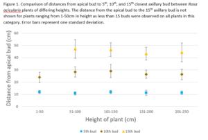
I have collected all of the data for my study on wild rose axillary bud spacing. I generated a figure for Small Assignment 5 to visualize key data. This figure displays plant height (the predictor variable) on the x-axis and the distance from the apical bud to the axillary buds (response variable) on the y-axis.

I originally had planned to show the distances for all 15 buds in the figure for each plant height category. I discovered that when all of this data was included the figure was messy and hard to interpret. By reducing the number of buds displayed to 3 (the 5th, 10th and 15th bud) visualization of the data points and error bars in clear. The inclusion of the data from the 5th, 10th, and 15th bud is a good representation of the full dateset and is sufficient to provide an appropriate visualization. The data from the other buds not represented in this figure may be displayed in a table in the report.

The creation of the figure provides supportive evidence for the prediction that axillary bud spacing is consistent regardless of plant height. The figure shows that at the 5th, 10th, and 15th axillary bud, the distance from the apical bud is easily within one standard deviation for all plant heights and no clear trends are displayed. These results suggest that there is an optimal spacing between the axillary buds for wild roses. For future research it would be worthwhile to further investigate what features have been optimized in wild rose crown architecture and what factors influence these features. For example I would like to investigate leaf size and location to measure the extent of self shading.

Percy Herbert Blog Post 7: Theoretical Perspectives

My research project is an observation of vegetative bud spacing in wild roses (Rosa acicularis).My hypothesis is that the physical spacing between vegetative buds on Rosa acicularis at the Queen Elizabeth Park duck pond is unrelated to the height of the individual plants. My prediction is that spacing of vegetative buds will be consistent for individual Rosa acicularis plants of all heights. I believe that this will be the case as I believe there is an ideal spacing between the buds as to maximize the amount of sunlight exposure to leaves. I predict tall plants will have vegetative buds in the same density as shorter plants as all plants will follow the same ideal spacing at their highest regions to maximize sunlight capture. The optimal vegetative bud spacing should be determined by maximizing leaf surface area at the highest regions of the stem while limiting self-shading. Plants must balance the above factors with the energy cost of producing supporting branches to most efficiently use carbon resources to position foliage in a process referred to as crown architecture.

Key Words: Self-shading, Light Capture, Crown architecture

Percy Herbert, Blog Post 6: Data Collection

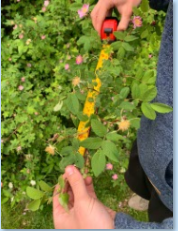
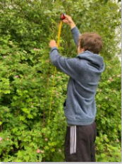
I was able to collect measurements on 50 replicates at the Queen Elizabeth duck pond.  50 individual wild rose plants (Rosa acicularis) were observed. Ten replicates were recorded in each of the five height categories (1-50cm, 51-100cm, 101-150cm, 151-200cm, and 201-250cm). The heights of the plants were recorded as well as the distance from the apical bud to each of the first 15 vegetative buds.

Measurements were much more difficult to collect this time compared to the first data collection as the vegetative buds have all sprouted into small branches containing leaves and flowers. The new growth is all a vibrant green colour while the original stems are a rich red colour so it is still easy to tell the difference between the new growth and the stem. The new growth made seeing the measuring tape and the junctions of the new growth and the stem much harder. Although the measurements were harder to collect, with added time accurate measurements were still possible.


One issue with data collection is that for some of the shorter plants observed there were less than 15 buds. This is especially true for the 1-50cm category. This may lead to the exclusion of this category in some of the data analysis steps.

Initial data analysis appears to support the hypothesis. The spacing between the buds does not seem to be altered by plant height. An ANOVA will have to be conducted to confirm this observation.

Percy Herbert, Blog Post 5: Design Reflections

For my sampling strategy I opted for haphazard sampling of individual rose plants. For the initial data collection in Module 3 I selected one plant in each of the following height ranges: 1-50cm, 51-100cm, 101-150cm, 151-200cm, and above 201cm. The reason why I have opted for haphazard sampling over random or systematic is that the area where the roses are located is specific and not large. Dividing the land into quadrats would also be exceedingly difficult due to the thickness of the roses and surrounding underbrush.  There are many unbranched wild rose plants that fall within each of the height ranges outlined above. Therefore it was easy to find one from each height range to observe for the initial data collection. The only difficulties in sample collection are the thickness of the underbrush making it tough to access the roses, and that the vegetative buds are beginning to form into leaves and small branches.

The initial data was not overly surprising. The sample size was much to small to derive any meaningful conclusions, however, the initial data supported my theory that the spacing of the vegetative buds is not related to the height of the plant. I also collected data on the number of vegetative buds on each individual plant and the distance from the apical bud to the lowest vegetative bud. These additional pieces of information did not provide any interesting information and I do not believe that I will continue to collect these data as I move forward with this experiment.

I plan to continue to use the same sampling method in an equal number of individual plants will be observed in each height range. I believe that by simply haphazardly observing many more individual plants in each height range I will be able to have enough measurements to perform an ANNOVA analysis.

Post 3: Ongoing Field Observations

Date: 18 May 2021
Weather: Mostly Cloudy, no wind, no precipitation
Temperature: 12°C

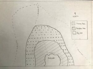
I returned to my field study site and made my way to Mundy Lake. Mundy Park has lots of western Sword Ferns throughout the park yet near the lake there were very few. As I made my way away from the lake, I noticed the soil became drier and the number of Sword Ferns slowly increased. This environmental gradient sparked my curiosity and I decided that this area would be my location for my field study. I used Google Maps on my cellphone to mark GPS coordinates in order to map out this environmental gradient.

1. Identify the organism or biological attribute that you plan to study.

Western Sword Ferns.

2. Use your field journal to document observations of your organism or biological attribute along an environmental gradient. Choose at least three locations along the gradient and observe and record any changes in the distribution, abundance, or character of your object of study.
EnvironmentalGradient
Environmental Gradient

Near Mundy lake it is marshy, and the soil is consistently wet. This area had very few Western Sword Ferns. As I moved away from the lake the elevation increases slightly and the soil becomes more dry and solid. Along this gradient, the number of western sword ferns increased with increased distance from the lake. The greatest number of sword ferns were found in the dry soil and the lowest amount was found in the swamp area.

3. Think about underlying processes that may cause any patterns that you have observed. Postulate one hypothesis and make one formal prediction based on that hypothesis. Your hypothesis may include the environmental gradient; however, if you come up with a hypothesis that you want to pursue within one part of the gradient or one site, that is acceptable as well.

Process

The underlining process that may be behind this pattern is the amount of water in the soil. The soil I observed across this gradient included dry, muddy, as well as standing water.

Since sword ferns are preferentially located farther away from the lake, I hypothesize that soil moisture is a determining factor in the concentration of sword ferns in this area of Mundy Park.

 Hypothesis

Sword Fern density is greater in soil that relatively dry and solid rather than saturated mushy soil or standing water.

Predictions

Sword Ferns are more likely to develop in areas wherein areas that are not marshy.

Sword Ferns are more likely to develop farther away from the lake.

Sword Ferns are more likely to develop in nutrient-rich soil.

4. Based on your hypothesis and prediction, list one potential response variable and one potential explanatory variable and whether they would be categorical or continuous. Use the experimental design tutorial to help you with this.

Potential response variable: occurrence of Sword Ferns (Categorical).

Potential explanatory variable: Soil moisture defined as solid, spongy, standing water (Categorical).

This study would be tabular since both variables are categorical.

Blog Post 4 – Sampling Strategies

For the tree sampling program, the three different sampling methodologies chosen were area-based random, systematic, and haphazard sampling. The most efficient methodology was random sampling, which was 20 minutes faster to complete compared to haphazard sampling (12 hours 8 minutes versus 12 hours 28 minutes). Systematic sampling was the most accurate for estimating diversity, with a Shannon-Wiener diversity index value of 1.5, which is the same at the true value. Random sampling was the least accurate, with a value of 1.3

The two most common tree species in the study area are eastern hemlock and sweet birch. Systematic sampling was the most accurate in estimating density of eastern hemlock, with a percentage error of 11.5% compared to random (18.4%), and haphazard (21.5%). Random sampling was the most accurate in estimating density of sweet birch, with a percentage error of 0.08% compared to haphazard (6.4%) and systematic (21.7%).

The two most rare species in the study area are striped maple and white pine. Both random and systematic sampling methodologies failed to record this species, while haphazard was fairly accurate in estimating density with a percentage error of 4.6%. All methodologies were poor at estimating density of white pine. Systematic was the most accurate with a percentage error of 90.5%, while haphazard had a percentage error of 247.6%. Random sampling failed to record this species.

The accuracy of density estimates declined the more rare the tree species were. Twenty-four sample points were likely not a sufficient number as multiple methodologies had large discrepancies between estimated and actual densities of multiple species, while some methodologies failed to record some species at all.

Percy Herbert, Blog Post 4: Sampling Strategies

The three sampling techniques used in the virtual forest tutorial were haphazard, random, and systematic. There are advantages and disadvantages to each of the three sampling techniques. For each of the techniques 25 area quadrats were observed. For haphazard sampling 5 quadrats were selected from each of the 5 topographical regions by trying to hand select quadrats representative of the average tree density in each region. For random sampling a random list of 25 coordinates were generated and those quadrats were observed. For systematic sampling a transect which crossed the entire sampling area, passing through all topographical regions was used. Quadrats were observed on alternating sides of the transect.

The quickest sampling method was systematic sampling at 12 hours and 36 minutes. This makes sense as there is little time spent walking between quadrats as they are all located in a linear line. Haphazard (13 hours 2 minutes) and random (13 hours 13 minutes) sampling both took longer than systematic sampling due to the distance between observed quadrats.

Systematic sampling was the most accurate sampling method for the 2 most common tree species (Eastern Hemlock and Red Maple). Systematic sampling had an error of 5% for Eastern Hemlock  density and 25% for Red Maple density, both lower than haphazard (14% and 51% error respectively) and random sampling (17% and 32% respectively). This result is expected as systematic sampling forces the observer to follow a preset system during sampling eliminating the possibility of the observer biasing the samples as can occur during haphazard sampling. Systematic sampling is also a more accurate predictor of the frequency of the two most abundant tree species then random sampling as 5 quadrats are selected from each topographical area. Random sampling allows for quadrats to be selected from any topographical region without any constraints on topographical regions.

Accuracy was better for all 3 sampling techniques for the higher abundance species then for the lower abundance species. Error for the density of the two least abundant species (Striped Maple and White Pine) were 60% and 100% for systematic sampling, 77% and 52% for random sampling, and 31% and 52% for haphazard sampling respectively. A small change in number of individual trees of a certain species can dramatically change the predicted density when the abundance is low. This is understandable as to get accurate results for the low abundance trees, more quadrats would need to be observed.

For predicting densities of tree species in this study it appears that systematic sampling has given the most accurate results. However, even with the use of systematic sampling, more quadrats must be observed if the densities of the lower abundance species are to be accurately predicted.