Since the field experiment that I designed and based my research around was fairly straightforward and simple, I did not have many difficulties in carrying out data collection or analysis. I did not make any changes from my original design that I drafted back in April as the abundance of mature western redcedar trees in the research area did not change between the spring and late summer when my analysis and report were concluded. There are aspects of field work that I had never considered before completing this project, and it definitely allowed me to appreciate the meticulous record keeping that must be done when large experiments and observations are being conducted. The work that is done by ecologists to preserve mature stands of forest is incredibly important and this research has made me acknowledge just how much work and dedication the ecologists have put into the conservation of the natural world and our understanding of it.
Category: Percy Hebert
Blog Post 9: Field Research Reflections
At the beginning stages of my field research project, I took a day or two to choose my research topic and my first observations of the area went smoothly. Since my sample area was located in my backyard, time was never a factor with my field data collections. However, the further I got into this project, the more difficulties I faced. An important lesson that I learned was that not all potential explanatory variables will be easily collected, examined or measured. I found this when I was deciding on how to represent and measure the effects of pH on Common Fern Moss percent cover. I was unable to easily measure the pH of the dead and healthy portions of grass and I was unable to think of a way to represent this data while displaying the relationship between pH and absence/presence of Common Fern Moss. I had to work around this problem by resorting to research articles touching on this relationship instead. In terms of the design of my project, I had to make a few adjustments along the way which weren’t too problematic. For example, I changed my quadrat size from 1m2to 0.25m2in order to minimize the amount of overlap between quadrats, and by doing this I had to recollect data on the first five quadrats I placed in the yard (which wasn’t an inconvenience as I had to collect data on 10 additional quadrats anyways…). Enrolling in this course and carrying out this research project on my own has not only altered my perspective on this practice, but has also increased my appreciation for the time and effort put in by ecologists to understand ecological processes and patterns. Conducting a research project isn’t easy, and from my experience, I believe it is a task that requires quite a bit of patience and an optimistic and open mindset.
Post 8: Tables and Graphs
I did not have any difficulties summarizing my abundance data in a simple bar graph, categorized by the three kinds of soil upon which my hypothesis is based. I graphed the relationship between the soil texture at each site along my environmental gradient and the abundance of individual trees sampled. The outcome supported my hypothesis that western redcedar trees would dominate areas of loamy soil that have better moisture-retaining properties than the sandy sites. The bar graph neatly summarizes the presence and absence of the three main species of the area: western redcedar (Thuja plicata), Douglas fir (Pseudotsuga menziesii), and ponderosa pine (Pinus ponderosa). The data did not reveal anything unexpected, but it inspired me to look into why western redcedar was completely absent from the sandy site (site 1) but was represented in the silty site (site 3). This prompted me to research competition between species in the interior cedar-hemlock biogeoclimatic zone, specifically between shade-tolerant and shade-intolerant species. It also inspired me to think critically about the overlapping niches of each species and how their evolutionary history has played a role in the spatial distribution of individuals within a mature stand.
Blog Post 8: Tables and Graphs
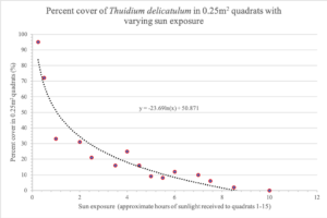
Above is the table I submitted for the fifth small assignment submission. It plots the relationship between the percent cover of Common Fern Moss, Thuidium delicatulum, and the degree of sun exposure in my yard. In order to create this graph, I had to measure the sunlight intensity of all quadrats (1-15) for every hour starting at 6:00 am and ending at 7:00pm on July 26th, 2019. Then, I sampled each individual quadrat for percent cover of T. delicatulum. I had some difficulty trying to categorize and separate each quadrat by the number of hours of sunlight received throughout this 13-hour time period. I eventually decided to basically approximate the relative amount of sun exposure received by each quadrat and used these values for the domain of this graph. When I put the graph together, I was very pleased to see that it follows my prediction (minus some outliers). I originally suspected that the graph of these two variables would be inversely proportional, and this graph mimics that trend. One of the outliers located at point (4,25) really stuck out to me because this quadrat happens to be located in a section of my yard in between the Japanese Lilac Tree and the Columnar Aspen. This area receives minimal sunlight and I recognized the soil in this area to be relatively moist when I was sampling in Module 2. Being that it is too difficult to go about sampling and representing soil moisture with the limited tools and resources I have at home, my best bet in inquiring about this specific observation would be scientific articles on this subject. I am curious to see if there are any scientific articles/studies out there that touch on the relationship between soil moisture and moss abundance. This would help for further exploration and answer a few questions I have going forward.
Blog Post 6: Data Collection
Field data collection activities: I got my Dad to record the values while I measured them. We located each of my replicates, measured width of branches at base to look for any limited growth patterns between the crowded and spaced replicates. We sampled buds with a 0.25m2 quadrat.
How many replicates: 30 in total, 10 per site
Problems implementing sample design: the quadrat: although I still believe was the best way to collect bud abundance, may have a moderate percent error. It was hard to count all the buds present in the quadrat because it is only 2 dimensional and there were some buds further behind those on the surface that still fell within the quadrat. I realize that the quadrat is more precise when placed flat on the ground, but this method was the only thing I could think of that would be somewhat accurate.
Ancillary patterns that caused hypothesis reflection: realized that all replicates are within the same soil conditions, very close proximity, so that wouldn’t be a major contributing factor to differences in growth, however, those in areas of high density might experience more competition for those soil resources.
Blog Post 8: Figures and Tables
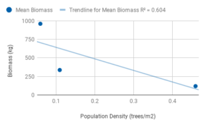
I decided to plot the relationship between population density and biomass of white spruces (n=30) that I found in my data. I calculated the biomass of all 10 replicates for each of the three sites (population density=0.46, 0.11, 0.06) using diameter at breast height (DBH;cm) and height (m), then calculate the mean for each site and plot it against population density. I originally wanted to plot all the biomass values, however I had trouble figuring out how to graph them due to the nature of my independent value. If I were to group the biomass values in terms of density, I am not sure how I would be able to compare the groups to each other. The outcome was generally as I expected, however it was less linear than I thought it would be. As you can see, my R squared value is only 0.604, so it is not a great fit for my data.
Post Nine: Field Research Reflections
Designing a field experiment is a mix of creativity, theory and adventure. While I love working in the outdoors and examining the natural world, any field research done over the winter limited daylight hours, plant identification and comfort while collecting data and observations. Extending the course into the spring allowed me to more holistically study Cates Park and its perennial plants and deciduous trees.
I changed my design a few times, including how data was collected, for realistic methodology, and to adapt to the knowledge and tools that were at hand. The changes are reflected throughout these blog posts and within the final project submission
Engaging in an ecological study has opened my eyes to the interdisciplinary subject matters integrated in ecology, as my subjects and connections in the study of nurse logs at Cates Park included Indigenous and logging history, ethnobotanical uses of local berry plants, conservation and public wellness. The vast amount of knowledge that is curated and studied in order to understand ecological processes is impressive and overwhelming, with so many variables that ensure this science will never rest as the world’s climate, biosphere and human values evolve.
Blog Post 7: Theoretical Perspectives
My research touches on biotic and abiotic factors, physiological stress, chemical stressors, and the stress-exposure-response model (SER model). Biotic factors are brought up in my experiment because my research examines the influence a living organism has on another. My dog has a direct influence on the grass because the urea from her urine becomes toxic and creates dead spots in my yard. Urea, combined with shade and moisture, all play the role of abiotic factors that influence the condition of Common Fern Moss (Thuidium delicatulum). When these nonliving agencies reach a suboptimal level, Thuidium delicatulumfaces physiological stress through restricted growth or rotting. Urea has a similar effect on the grass in my yard. Increased exposure of urea causes toxicity to the grass and kills it. These cause-effect relationships mentioned above allude to the SER model (stress-exposure-response). The SER model demonstrates the biological or ecological changes as a result of the change in intensity of environmental stressors.
Three keywords that I could use to describe my research project are: chemical stressors, percent coverage, and abiotic factors.
Blog Post 6: Data Collection
Due to the size constraint of my backyard, I decided to modify the size of original and additional quadrats. I decided to decrease the size to 0.25m2 in order to prevent the chance of overlap between replicates and to hopefully receive more accurate data in the process. In my initial data collection, I sampled at five locations using 1m2 quadrats. The three locations that I observed for my ongoing field observations are each unique from one another in terms of sun exposure throughout the day, the presence of dead grass and soil moisture. I then decided that the best way to select my first five replicates was to use the Stratified Random Sampling technique. I took one replicate from Location 1, another replicate from Location 2, and three replicates from Location 3. Using these replicates, I measured the percent cover of Common Fern Moss (Thuidium delicatulum) relative to a 1m2 quadrat size and used this data as a measure of abundance for this type of moss. Then, I calculated the mean percent cover of Common Fern Moss in these quadrats to get an idea of the area of my yard occupied by moss. I collected data on five additional replicates and had to recollect data from the original five plots using 0.25m2 quadrats. I had to resample the first five replicates because by decreasing quadrat size, the percent cover was expected to increase relative to the quadrat. This prediction was for the most part correct, as all values for the percent cover increased with decreasing quadrat size except for quadrat 5, where the value remained the same.
At this point, I have noticed a general trend in my data (with a few outliers) that supports my prediction and I have not yet reconsidered my hypothesis. I am seeing that areas in my yard that would typically receive more sunlight throughout the day have a smaller percent cover of fern moss in comparison with quadrats that receive more shade. My second data collection was in my mind successful, however, I hope that I can find a way to measure pH in these 10 and additional quadrats in order to factor in the impact of soil acidity on moss growth- I am sure I will find a way to go about that before my next data collection.
Blog Post 8: Tables and Graphs: Cates Park
Although I intend to focus on the success of Tsuja heterophylla on nurse logs versus the forest floor, I collected data on the presence and absence of all species found within the quadrats I studied in four regions of Cates Park in North Vancouver. Limiting the data to one species in a chart helps with the ease of interpretation, but limits the understanding of species richness in the microsuccessions of nurse logs versus the forest floor. Organization was simple due to the presence and absence data collected, and would have been more difficult had I included other species present. I will likely discuss this in my final paper to address the succession species found in Cates Park. The outcome was as I expected: Tsuja heterophylla were present more often on nurse logs than not. Further exploration could include canopy cover in relation to this tree’s success or competition with other species in the region.
