Blog Post 3 – Ongoing Field Observations

Date: 8 May 2021
Weather: clear, no wind, no precipitation, 10% cloud cover
Temperature: 7°C

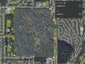
I returned to my proposed study area on 8 May 2021 at 0700. The first habitat type I travelled to was the forested area. Immediately I noticed more birds singing than the previous week. I looked at two different locations within the forested portion, and then travelled to the open portion of the study area. I left site at 0759.

Location 1: 10U 439505 / 5425195

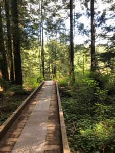
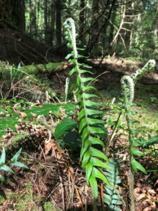
This location is in the southwestern portion of the proposed study area. It is dominated by young coast Douglas-fir (Pseudotsuga menziesii var. menziesii) and has a moderate amount of understory consisting mostly of salal (Gaultheria shalon) and sword fern (Polystichum munitum). The canopy closure is approximately 65%. The following bird species were recorded at this location:

  • Townsend’s warbler (Setophaga townsendii)
  • Pacific wren
  • Red-breasted nuthatch (Sitta canadensis)
  • Brown creeper (Certhia americana)
  • Chestnut-backed chickadee
  • Pacific-sloped flycatcher (Empidonax difficilis)
  • Northern flicker (Colaptes auratus)

Location 2: 10U 439671 / 5425085

This location is in the southern portion of the proposed study area. It is similar in vegetation to Location 1, but it is on a steeper slope. The canopy closure is approximately 60%. The following bird species were recorded at this location:

  • Townsend’s warbler
  • American robin (Turdus migratorus)
  • Golden-crowned kinglet (Regulus satrapa)
  • Northern flicker
  • Pacific-sloped flycatcher

Location 3: 10U 439687 / 5425356

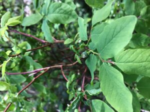
This location is in the northwestern portion of the proposed study area. Vegetation is dominated by scotch broom (Cytisus scoparius), with lesser amounts of salal and a few red alder (Alnus rubrus) and vine maple (Acer douglasii) saplings. Although birds were still singing, compared to the forest there appeared to be a lesser amount. The following bird species were recorded at this location:

  • Spotted towhee (Pipilo maculatus)
  • Song sparrow (Melospiza melodia)
  • Dark-eyed junco (Junco hyemalis)
  • White-crowned sparrow (Zonatrichia leucophrys)
  • American robin

My hypothesis is that songbird species richness and abundance is impacted by structural stage of habitat. I predict that songbird species richness and abundance will be higher in the forested portion of the study area rather than the open, shrub-dominated area.

Response variables will be songbird species richness and abundance. The explanatory variable will be structural stage. The response variable would be continuous, while the explanatory variable would be categorical as structural stage is based on a limited number of values.

Blog Post 2: Sources of Scientific Information

The Source:

The source of ecological information that I chose is a recent paper published in the Journal of Ecology called “Quantifying nectar production by flowering plants in urban and rural landscapes”.

Type of Information:

This Source is Academic, Peer-reviewed, Research material.

Support for this Classification:

Academic:
This article is considered academic since the authors are experts in their fields which includes Faculty and a Ph.D. Students from the University of Bristol. All the authors have a high level of education in this field and work in established universities. The Articles also use in-text citation as well as a reference section on pages 1755-1757 which further supports that this article is academic material (Tew et al., 2021).

Peer-reviewed:
This article is peer-reviewed since it was published in a peer-reviewed academic journal called the “Journal of Ecology”. The article also has a section titled “Peer Review” on page 1755 where there is a link to the journal’s website (Tew et al., 2021). On the journal’s website, it states that this article was peer-reviewed by reviewers and by Ignasi Bartomeus with supporting documentation of the review processes that took place before this article was published.

Research:
This article is research material because there is a material and methods section on page 1748 (Tew et al., 2021). This section outlines how the data was collected and the sampling method.

References:

Tew, N. E., Memmott, J., Vaughan, I. P., Bird, S., Stone, G. N., Potts, S. G., & Baldock, K. C. (2021). Quantifying nectar production by flowering plants in urban and rural landscapes. Journal of        Ecology, 109(4), 1747–1757. https://doi.org/10.1111/1365-2745.13598

Blog Post 2

Verschuyl, J., A. Hansen, D.B. McWethy, R. Sallabanks, and R.L. Hutto. 2008. Is the effect of forest structure on bird diversity modified by forest productivity? Ecological Applications, 18(5):1155-1170.

https://www-jstor-org.ezproxy.tru.ca/stable/pdf/40062219.pdf?refreqid=excelsior%3Ae45ea5077ddaa99c33964d7c2f1828d2

The paper is academic, peer-reviewed research material. The paper contains in-text citations and a bibliography making it academic material. The paper occurs in the Ecological Applications journal which is published by the Ecological Society of America. As per their website, all accepted manuscripts go through the peer-reviewed process (ESA 2021). The paper contains field data which has been analyzed, making it research material rather than review material. A quick google search indicate numerous relevant papers have been written by these authors, demonstrating their expertise in this field.

References:

ESA (Ecological Society of America). Peer Review Process. [accessed 2 May 2021]. https://www.esa.org/publications/peer-review-process-overview/

Blog Post 1

Date of Site Reconnaissance: 2 May 2021
Weather: Partly Cloudy, no precipitation
Temperature: 14 degrees Celsius
Season: Late Spring

A site reconnaissance was completed at the proposed study area which is located immediately west of Ladysmith, BC (Figure 1) on 2 May 2021 from 1345 to 1423.  The area is approximately 0.36 km2, with an elevation range of 115 m to 190 m above sea level (asl), with an average elevation of 145 m asl. The study area overlaps with municipal land and provincial crown land and falls within the Coastal Hemlock very dry maritime (CWHxm) biogeoclimatic zone (Government of BC 2021). The study area is comprised of two general habitat types: second growth coniferous forest and open, tall-shrub habitat. It is bounded to the west by Holland Creek and the Ladysmith water filtration facility, to the north by a rocky ridge, and to the south and east by additional clear-cuts (Figure 2). The study area was derived this way so the two available general habitat types were approximately equal in size.

Figure 1: General Location of Study Area

Figure 2: Study Area

The second growth coniferous forest is dominated by coast Douglas-fir (Pseudotsuga menziesii var. menziesii), with western hemlock (Tsuga heterophylla) and western redcedar (Thuja plicata) being the sub-dominant tree species. The understory is dominated by salal (Gaultheria shallon), with lesser amounts of vine maple (Acer circinatum), oceanspray (Holodiscus discolor var. discolor), and red alder (Alnus rubra) (Photograph 1). The forest is somewhat sloping, with a steeper gradient to the west. This area has a canopy closure of approximately 60 % and a moderate amount of coarse woody debris. The following bird species were recorded in this habitat type during the site reconnaissance:

  • Townsend’s warbler (Setophaga townsendii)
  • Pacific-slope flycatcher (Empidonax difficilis)
  • Pine siskin (Spinus pinus)
  • House finch (Haemorhous mexicanus)
  • Orange-crowned warbler (Leiothlypis celata)
  • American robin (Turdus migratorus)
  • Brown creeper (Certhia americana)
  • Red-breasted nuthatch (Sitta canadensis)

Photograph 1: Example of second-growth coniferous forest portion of study area.

The open tall-shrub habitat falls within a right-of-way for a transmission line as well as an additional cleared space (Photograph 2). Vegetation is largely dominated by scotch broom (Cytisus scoparius), with lesser amounts of sapling vine maple and red alder, and some small patches of salal. A few mature bigleaf maple (Acer macrophyllum) are also present, but generally the area has no canopy closure. The area has minimal coarse woody debris and is generally flat. The following bird species were recorded in this habitat type during the site reconnaissance:

  • Spotted towhee (Pipilo maculatus)
  • Dark-eyed junco (Junco hyemalis)
  • Anna’s hummingbird (Calypte anna)
  • Rufous hummingbird (Selasphorus rufus)
  • American goldfinch (Spinus tristis)
  • American robin
  • Northern flicker (Colaptes auratus)
  • White-crowned sparrow (Zonatrichia leucophrys)
  • Song sparrow (Melospiza melodia)
  • Turkey vulture (Cathartes aura)

Photograph 2: Example of open, tall shrub habitat portion of study area.

Three questions that arose from the site reconnaissance are as follows:

  1. Which habitat type has a higher bird species richness?
  2. Which habitat type has a higher bird abundance?
  3. Do invasive vegetation species have a detrimental effect on local bird populations?


References

Government of BC. 2021. iMap Mapping Tool. [accessed 2 May 2021]. https://maps.gov.bc.ca/ess/hm/imap4m/

Blog Post 1 – Observations

Date/Time:

Visited the site on May 1, 2021, at 16:00.

Weather:

The weather was partly cloudy with no precipitation. The temperature recorded at the site was 17oC. The seasonality is Mid Spring.

Observation Area:

The area that I have chosen to observe is the forested portion of a City park in Coquitlam, BC called Mundy Park. This park is 1.39 km2, has two lakes, is flat and mostly forested.  The park is surrounded by dense suburb developments, and the park trails are a common area for dog walkers and runners.

Figure 1. Satellite View of Mundy Park

Observations:

While walking through the park I noticed that there were different plant species that appear to thrive near the lakes when compared to other regions of the park. My main focus was the abundance of plant species near Mundy lake which is more centrally located in the park and more accessible. The forest seems healthy with few invasive species identified in the central areas of the park. Some of the plant species that I was able to identify are shown in the figures below.

lakeside loop trail
Figure 2. Lakeside Loop Trail
Western trillium
Figure 3. Western trillium
Salal
Figure 4. Salal Near The Lake
Oval-leaf Blueberry
Figure 5. Oval-leaf Blueberry
Western sword fern
Figure 6. Western Sword Fern

Questions

  1. Which areas of the park have the greatest number of Oval-leaf Blueberry and what are the reasons? (sunlight?)
  2. Does proximity to Mundy Lake correlate with a change in the plant species that exist in the area?
  3. Does the proximity to the homes and roads surrounding the park result in a higher number of invasive plant species? (Does the perimeter of the park has more invasive species?)

Blog Post 8: Tables and Graphs

My project involves looking at the surface density of springtails (Collembola) in response to the presence or absence of cover. The data collection consisted of counting individual arthropods on the snow surface within 10 quadrats in two treatments (5 each), three times a day, over the course of five days. So though I had 150 data points, I organized them into 10 rows (corresponding with the quadrats) and divided the data up into columns according to their respective categories (date, time of day, treatment) in Excel and found this visually easy to manage. However, trying to analyze these data points in Excel was not as straightforward, partly because I’m no expert at Excel as a data management tool, and partly because “visually easy to manage” seems to be more of an endpoint of data analysis (the table or graph) rather than a starting point of data management. My “data whiz” friend informed me that data input is easiest to manage when each data point has its own row (in my case that meant 150 rows) and is only located in one column, and to try to ensure that the rest of the data (treatment, date, time-of-day) is specific to its own column – even though that means that the values within these cells would get repeated. This information allowed me to at least partially understand the way a program like Excel reads data, and I began to see how powerful a tool it can be to process, analyze, and display data, especially when datasets are large.

The graph I produced with Excel showed me that there definitely was a trend in my data, possibly a significant one. Though I need to run a p-test to see if I can reject the null hypothesis (the standard error bars between treatments appear to almost overlap), there certainly appeared to be a springtail preference for full sunlight rather than cover. This is the opposite to my prediction of a preference for shade based on observation, as well as the shade preference seen in the results of certain experiments done in the literature (Salmon and Ponge 1998). However, upon further researching this fascinating order of arthropods, I’ve come to understand that there are over 5000 species, some of whom live their lives totally subterranean, some of whom live in surface layers of soil and organic matter, and some of whom live above ground and with a multitude of life strategies and abiotic tolerances (Hopkin 1997).

The small graph I was able to generate from my data reveals to me that my experiment would most certainly be improved with more replicates done over a greater time span and in different habitats. Having more expertise at species identification and sampling in different habitats would also provide more robust scientific knowledge to the ecology of Collembola, as different species likely have different preferences for light and darkness depending on life events that may be occurring at different times throughout the winter (rearing, migration, reproduction etc.).


References:

Hopkin, S.P., 1997. Biology of the Springtails (Insecta: Collembola). Oxford University Press, Oxford.

Salmon, S., Ponge, J.F. Responses to light in a soil-dwelling springtail. European Journal of Soil Biology 34: 199-201.

Post 9: Field Research

While conducting the field research on moles and their predators,  I learned a great deal more than I expected about research techniques and ecology.

It was necessary to change my design a few times, as I acquired feedback from my instructor. Primarily the adjustments included how to conduct the samples in an accurate manner, and how to gather data efficiently while ensuring replicates were conducted to limit the possibility of errors due to small sample sizes. In retrospect I may have complicated my project by selecting a predator and prey model rather than something more simplistic such as non moving organisms like grasses or lichen in microhabitats. Regardless the challenge (and fun) was to find a way to sample my communities accurately.

Participating in this course and engaging in these activities has given me an appreciation for ecology.  The rich complexities of how sampling, research, statistics, natural history, geography and even geology are brought to bear on a problem.

While I do not consider myself an ecologist, I have enjoyed the process and will likely look at the natural world differently now. The blessing in all of this has been that I have learned some basic tools on how to see how communities interact and have a new found appreciation for ecology.

Blog Post 8: Tables and Graphs

After entering my data into excel I found that it was difficult to display the data as a whole without breaking out the separate data sets gathered. Since I had gathered information on predators and a separate group of data on prey, I had to find a way to display this in a way that showed the relationship. Eventually I settled on the average of the number of signs of predator activity and also the average number of signs of prey activity.

The result in graph showed an immediate trend between the two, and I was pleasantly surprised to see how clear the relationship was. However, I also had to reconcile that I had gathered only a single weeks worth of data from 35 point counts (Conducted each day). While there was a lot of separate data to draw from I realized that a longer term study over a month or two in less areas may have given my data more weight and allowed me to see a more longer term trend such as is predicted in Lotka-Volterra models.

Overall, even with a shorter time duration of data gathering, I came away with a better understanding of why long term studies really hold alot more weight than shorter duration studies.

Blog Post #7: Theoretical Perspectives

In reviewing the theoretical perspectives of my project, I have had to combine observational activities with literature review to gain an understanding of the behaviour within my species of study. My study is looking at the presence of snow fleas (springtails in the order Collembola) on the surface of the snow in response to open-sky vs. shaded situations. I observed the way they jumped around above the surface but also the way they were able to disappear into the snow and presumably move about within the snow column. Although they weren’t evident in large numbers during my data collection period, I have witnessed them in extraordinary numbers peppering the snow at warmer times throughout the winter months. As Hagvar (among others) note, different circumstances may account for these large-number events including the need for migratory dispersal in temporary or patchy habitat environments, or just changes in soil conditions during periods of melt, such as inundation of water on the surface of the soil. Being able to be mobile on the surface of the snow is a great advantage for organisms less than 1mm in size in any terrestrial landscape, but is especially useful for migration over bodies of water or rivers, which springtails have been observed to do. The ecological processes my hypothesis is based on concern both a springtail’s need for cover as a means of hiding from predators, and the need for having a view of the sun as a navigational tool in migratory circumstances during the winter.

Keywords:  Snow fleas, dispersal, sunshine

References:

Hagvar, S. 2000. Navigation and behaviour of four Collembola species migrating on the snow surface. Pedobiologia 44: 221-233. https://doi.org/10.1078/S0031-4056(04)70042-6

Percy Herbert, Post 3: Ongoing Field Observations

For my research study I am deciding to focus on vegetative bud formation on wild rose plants. I have observed that taller rose plants appear to have long stems with no vegetative buds forming until the upper portion of the plant. The density of the vegetative buds at the upper regions of the plants appear to be consistent regardless of the height of the plant and how long the barren stem is below the buds.

More specifically, I will be measuring the distance from the tip of rose plants to the first, third, fifth, tenth, and lowest bud on the stem. I will take measurements from many individual plants, each of which will be measured to determine the height of the plants. I will take measurement from non-branched plants ranging from under 50 centimeters to over 2 meters. I will then try to determine if there any observable trends relating the distance from plant tip to vegetative buds to the height of the plant.

My hypothesis for this study is: For wild rose plants in Queen Elizabeth Park, there is an optimal distance from the tip of the plant to vegetative buds, regardless of plant height.

My prediction: Once rose plants reach a certain height the lower section of the stem remains bare. The density of vegetative buds will be the same in the upper regions of short and tall rose plants.

The response variable: distance from tip of plant to the first, third, fifth, tenth, and lowest vegetative bud on the stem. (continuous)

The predictor variable: height of the plant (continuous). In my study I will trying to prove that the height of the plant is not the most important factor in determining the location of the vegetative buds on rose plants.

A regression study would be appropriate for this study as both the response and predictor variables are continuous.