Observation 3: Ongoing Field Observations

1.With switching locations, I’ve really had to brainstorm what I could study at this location. I’m quite interested in birds, but also vegetation. Upon observing this location, I found it interesting how the vegetation differs on one either side of the raise footpath considered the dyke, and the sides of the dyke. I’ve scanned some images below to highlight how the growth differs on each side.

2. That being said, I chose three parts of the dyke. The first is along the water with the left slant of the hill, the top of the dyke pathway, and the right slant of the hill along the farm border. From the water to the farm border is about 15 meters with 5 meters in between each spot.

3. Besides the different proximities to the water, I observed that the soil seems to be a little different. Particularly on the bramble side (left side) it was quite rocky with less concentration of dirt. Perhaps this is why grass does not prosper along that side? I also observed that around 14:10-14:48 in the afternoon, the sun does not shine on the left side. In fact, it was quite cool without the direct sunlight. When you compare plot A to plot B, the sun is direct, there seems to be a saturation of water in the soil (there was mud present). Plot C also seemed to have some saturation in the soil (a little soft), but not as much as plot B. Surprisingly, because plot A is along the water, although on the hill, there was not a lot of water present. Is this because the water directly runs off the hill and into the water?

I’d like to explore a hypothesis about the soil composition and how it supports the type of vegetation that grows on each plot as well as the amount of exposure of sun throughout the day on B and C.


My formal prediction: The soil composition along the dyke determines the variety of vegetation that successfully grows in each plot.

4. The response variable for this hypothesis would be the vegetation and it would be a continuous variable. The explanatory variables will be the soil composition and amount of saturation that contributes to the soil composition. This will be a categorial variable. I will use a one-way ANOVA experimental design for this study.

Post #3 Ongoing Field Observations

I have looked at a few ideas for study options up to this point. Most of my experience has been in forestry and vegetation, so a vegetation-based project was my natural first choice. The fact that it is winter here in northern BC and the ground is under a few feet of snow is one reason why looking at something other than plants is maybe a good idea. Here are some of my ideas up to this point:

I thought of looking at shrub abundance in relation to conifer crown closure, but this would require a truly landscape-level study.

I thought of looking at beaver presence-absence as a predictor for shrub and aspen-ramet abundance, but once again this would require being able to see evidence of beaver which would likely be under the snow.

I thought of looking at pine plantations and observing how young individuals grow bigger and taller in the presence of nitrogen-fixing shrubs such as alder than those individuals growing where alder isn’t so abundant.

What I’ve finally settled on is something truly fascinating and present in so many different environments in these parts – an organism I see all around my home as well as in the forests that I walk, ski, snowshoe, and work in. I will number the following points as per the blog instructions in order to keep everything easy to follow.

1) We (my family and the people around me) call them snow fleas but they are actually springtails, tiny arthropods that present themselves in different abundances all throughout the winter. In the order of Collembola, they come out on warm winter days and jump around on the snow and their bodies contain proteins that act like antifreeze to allow them to function in sub-zero temperatures (wikepedia). I would like to study their abundance and distribution in terms of density under different circumstances.

2) I will describe three environmental gradients in which I’ve observed them:

  • Open undisturbed snow in which (as of today March 7 2021) they were fairly uniformly and sparsely distributed.
  • Forested ground with crown closure where I saw they were quite a bit more dense, interspersed throughout bits of tree debris and forest matter
  • Disturbed snow, particularly relatively fresh disturbances like footprints from a few hours prior before new snow has fallen, in which they seem to congregate in large numbers, sometimes on one side of the footprint or the other which begs a couple questions. Are they seeking shade within the disturbance? Do they just happen to be in greater numbers because the disturbance has decreased the snow depth in that one place?

3.) As far as processes that may contribute to their relative abundance in different circumstances – open, closed or forested, and disturbed – there are likely several reasons:

  •  As they are soil organisms, they are likely present in greater numbers over-top of ground that is richer or more nutrient-dense.
  • Snow-depth probably has a part to play – I would predict that as snow depth decreases, springtail density would increase.
  • Under cover of trees and with other bits of forest matter and debris scattered on the snow they would have more camouflage and be less visible to predators.
  • Direct or indirect sunlight may have an effect on their abundance.


One hypothesis I would like to explore – one that I think would lend itself to a study that would be possible to implement – is this:

Springtail density on the surface of the snow is determined by the presence of direct sunlight.

One formal prediction based on this hypothesis:

Though sunlight contributes to a warming environment conducive to springtail emergence, springtail density will be higher under cover or under a source of shade.

4.) The response variable in this case would be the density of springtails – this is a continuous variable. The explanatory variable would be presence or absence of direct sun (i.e. sun or shade) – this is a categorical variable. For this study, the experimental design would be a one-way ANOVA.

Blog Post 7: Theoretical Perspectives

My field project study involves assessing the abundance of Broadleaf Stonecrop using percent cover in 1m2 quadrats along a few environmental gradients including elevation from sea level and micro habitat transition from shoreline to forest. My hypothesis is that Broadleaf Stonecrop abundance is determined by the moisture of the substrate which is indicated by a categorical level of drainability. Therefore I have predicted that the Stonecrop is most abundant in areas with high degree of drainability.

Thus far during my data collection I have noticed several ecological influences that may be affecting the abundance and distribution of my study subject. These would include exposure to sunlight, the underlying substrate, degree of slope within the growing area, substrate moisture content, as well as competition with other vegetation. 

Since the Broadleaf Stonecrop is  a succulent, they seem to thrive with very little substrate moisture hence my above prediction. They also thrive in areas where very few other vegetative species would be able to grow primarily steep, ocean exposed rocky outcrops along the shoreline. They also seem to require a high degree of sunlight and their abundance decreases dramatically in higher vegetated areas that would shade out the Stonecrop. Interestingly, it has been observed that the Stonecrop also only grows along the ocean facing cliffs in the study area, not the lagoon facing side.

Therefore both abiotic and biotic factors are having a direct and indirect influence on where the Stonecrop is most abundant. This study also touches upon competition for space and resources among various vegetation, adaptability in seemingly harsher environments, and higher tolerance for dryer conditions.

Three keywords that could be used to describe this study are climatic stressors, substrate moisture, and slope gradient.

Blog Post 5: Design Reflections

I have changed my study topic and will not be carrying out the study that I outlined in earlier blog posts.  My new study will also take place at the Richmond Garden City Lands.  During the implementation of my previous study I noticed that there was a man made walkway through the bog and that there appeared to be more abundance nearer the path.  I have decided to collect samples on a transect. I used five transect lines spaced 5-m apart.  Each transect began on the edge of the man made path and was walked 10-m East into the bog.  The transect was sampled at three random points (1-10 meters from the path).  At each point I placed a quadrant and identified the amount of vegetation covered using a 0.5-mx0.5m quadrant that was gridded to have 25 10-cmx10-cm squares.  I took the pH of from the centre of each quadrant to see if there was an association with pH and vegetation abundance as well.  


I thought that it would be a good idea to do the transect sampling randomly.  By laying out 5 transects and randomizing a number from 1-10 using the generator from random.org.  I have changed my mind on this and will be sampling systematically at three points spaced 5-m apart on each transect.  I decided to change this strategy to make sure that quadrants were not too close to each other so that I could be confident that these samples had independence.   


Collecting this data also made me realize that I lacked focus for a hypothesis.  I found that plant diversity had a more interesting pattern.  There was more plant diversity near the path than there was in the bog.  I think that this is because many plants are sensitive to slight changes in pH and the man-made path brought less acidic soil to the bog.  I think that this is why there is less species diversity further away from the path.  I believe that plant diversity will decrease as the soil becomes more acidic.  The transects will be used in the same design as described above but the predictor variable will be soil pH (or acidity) and the response variable will be plant diversity.

Blog Post 4: Virtual Forest Tutorial

I used the distance-based methods in the virtual forest tutorial.  Systematic sampling was the fastest, taking 4 hours and 15 minutes, random sampling took 4 hours and 38 minutes and haphazard was the slowest at 4 hours and 44 minutes. 

Random sampling had the most accuracy in regards to the two most common tree species and one of the rarer species.  Systematic sampling was the most accurate in regards to the rarest species (white pine).  The haphazard sampling method was not accurate in regards to both abundant and scarce species. 

The systematic sampling technique was more accurate with scarce species than common species and this could be due to the nature of distant-based sampling along one direction.  The systematic sampling method may have not been the most accurate in every species sampled but it did have the most accurate average overall and seems to be a more reliable method of sampling.


Sampling Technique % Error Eastern Hemlock (common) % Error Sweet Birch (common) % White Pine (rare) % Striped Maple (rare)
Systematic 9.9% 64.0% 1.2% 3.4%
Random 3.1% 47.4% 100.0% 0.5%
Haphazard 138.0% 142.9% 142.0% 16.5%

Blog Post 6: Data Collection

First day of sampling occurred on Saturday, Feb 27th at approximately 9:30am within the headland island of Pipers Lagoon, in Nanaimo B.C. 

Study Hypothesis: Broadleaf Stonecrop abundance is determined by substrate drainability.

For my first day, I sampled three replicates on the Western portion, and one replicate on the Northern portion of the headland island. Each replicate consisted of a 40m long transect with the starting point randomly placed above the high water mark along the backshore. I originally planned to do a 50m length but felt it was redundant to sample that far into the inland forest. I chose the heading of each transect to be approximately towards the center of the headland island. Each transect, therefore, covered the full environmental gradient from coast to inland forest.

Along each transect, I placed a 1m2 quadrat starting at 0m and then every 3m, for a total of 14 subsamples per transect. Within each quadrat, I recorded the elevation above sea level, the substrate type, the sloping characteristic (gradient), the percent cover of my study subject (Broadleaf Stonecrop), and the distance along the transect. I also made note of the amount of sun exposure specifically whether it was an open space, or shaded by other vegetation.

Overall my study design was effective, albeit somewhat time-consuming. To speed things up a bit I may take pictures of each quadrat and from those assess the percent abundance and substrate type. I did have to adjust the starting locations of a couple transects slightly to allow for safer access to points along the transect.

Generally, my data collected thus far does tend to agree with my hypothesis, although based on patterns observed, sun exposure does seem to also play an important role in the Broadleaf Stonecrop abundance.

I will continue to implement this study design throughout the remaining area of the headland island. This will require 2 more transects in the Northern portion and 3 each in the Eastern and Southern portions for a total of 12 transects (replicates).

Post 9: Field Research Reflections

Overall, I enjoyed this experiment and spending the amoutn of time observing that I did. I enjoyed getting out early each morning before work and observing the birds at the local natural park. There were far more species than I had seen there previously. There were times that I found it quite cold, of course. At times, being outside for an hour at 7am, in January, was really quite cold. But observing the patterns and species present, was really quite interesting. In hindsight, I think I would have implemented a different/better design or hypothesis. The location I had available to me was perfect for observations, but I could likely have chosen a better route for my study. The practice of ecology is more complex and involved than I had considered or realized previously, and I certainly have a higher appreciation for it having completed the course.

Post 5: Design Reflections

Previous data collection method

I used random.org for all my random number-generation. In my methods descriptions below, I will put the parameters for the generated number in brackets.

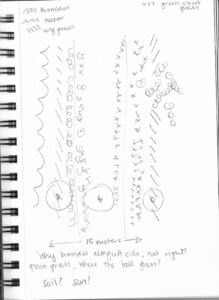
For my recent field observations, I decided to use simple random selection to choose sampling sites. I chose my starting point by walking 20 paces (10-30) north of the steps up to Volunteer Park. My process for determining the actual sample sites required me to be able to move in any direction, so it was important to have a starting point that was not on the edge of the beach.

Each new sampling site was chosen in a two-step process. I generated a number to indicate direction (1-4, where 1 = northwest, 2 = northeast, 3 = southwest, 4 = southeast), then generated a number of paces (5-15) to walk in that direction to take another sample. I repeated this procedure 10 times, more than the required 5, because the first five samples had no oysters at all (an early sign that the method would have to be modified).

At each sampling site, I recorded whether or not there was a large rock present (as a yes or no), and how many oysters I saw within the quadrat (oyster numbers broken down into two categories, attached and unattached).

Difficulties in implementing that sampling strategy

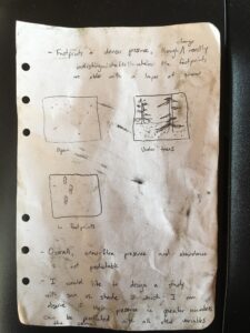
With my previous sampling strategy, each sampling site basically fell into one of four possible categories:

Notebook Scan on Feb 23, 2021 at 19_32_24


Almost all of my sampling sites were in the bottom right quadrant – they had neither rocks nor oysters. If I was seeking to measure the density of the oysters on the beach, those would be useful data points, but I am primarily interested in whether oysters are more likely to be near large rocks. Upon reflection, even the bottom left quadrant – rocks but no oysters – is not relevant either, because my question isn’t “are rocks more likely to have oysters nearby?” (which is superficially similar to “are oysters more likely to be near rocks?”).

I also was not leaving markers of where I had previously sampled, and my randomization method did not account for or prevent me from going back over previous areas. Since I was equally likely to go south or north, east or west, on average I was generally staying in the same place.

I diagrammed my movement using my notes, and it’s clear that some sampling sites were very close together. With more options for directions, eg. including north, south, east and west (so 1-8), I probably would have been less likely to ever immediately backtrack, but still equally likely to circle back to the same places. Although my previous strategy was random, I don’t think the sites were all sufficiently far apart to be independent.

Modifications to sampling strategy

Going forward, I will change how I randomize (for better independence) and what specific information I collect (to better address the research question).

Randomization

I will first measure out a section of the intertidal zone in paces, and then diagram it in my field journal. From there I can generate a set of x- and y-coordinates using random.org with the parameters I just measured. I’ll place those coordinates on my diagram in order, and eliminate any that are within a certain number of paces of a site that’s already on the map. I’ve drawn up an example of how this might look.

Data collection

At each sampling site, I will look for the nearest oyster. I will then record whether it is close to a large rock, or not. I believe this will better address the research question, because each oyster will be the sampling unit and the recorded information will then allow me to compare the number of oysters near rocks versus the numbers not near large rocks. To note any potentially confounding variables, I will also record whether that oyster is attached or not (in case attached oysters are more likely to be on rocks than unattached), and measure the oyster’s size.

Surprises in data collected so far

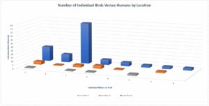
In the data I have already collected, using the previous sampling method, only four samples even had oysters present. Contrary to my expectations, half of the sampling sites that contained oysters did not have any large rocks. The most oysters found at one site (6) were found in a clear space without rocks.

I am not going to draw any conclusions from that information because, as discussed above, the method for collecting the data was flawed, and I don’t think four data points are sufficient.

Post 4: Sampling Strategies

Of the three sampling techniques (systematic, random, and haphazard) that I used for the virtual forest tutorial, the technique with the lowest average error rate was the systematic sampling.

The fastest technique was the haphazard sampling (12 hours 34 minutes), but the difference between the fastest and the slowest was only 13 minutes (1.7% of 12 hours 34 minutes), which is fairly negligible.

Screen Shot 2021-02-21 at 22.29.22

Common vs. rare species

The average error rate for the two most common species, Eastern Hemlock and Sweet Birch, was 18.1%. The average error rate for the two least common species, Striped Maple and White Pine, was 42.9%. From this dataset, it appears that the accuracy did decrease with species rarity.

Comparing sampling techniques

Systematic sampling had the lowest average error rate, at 16.7%. Random sampling had the highest average error rate, at 46.2%.

Based on this dataset, systematic sampling appears to be the most efficient and accurate. With systematic sampling, I found the lowest error rates (on average) with only a two-minute time penalty over the fastest technique. The 16% error rate average still seems high, to me, so I would want to re-do this exercise multiple times, probably with more samples, to be able to better identify the technique most efficient in this setting and its most efficient number of samples.

Post 8: Tables and Graphs

It is difficult to see the chart below, but it represents the values of individual birds documented, the number of humans/hikers that were present on that portion of the trail at that time, and it is separated by the three Locations A, B, and C which were observed. It did take some time for me to organize and rearrange my data into formats that would pull the information I was looking for. I did find it to be challenging, but also a learning experience. My data did reveal a few patterns that I was surprised by. It appears that the bird populations tend to be much more abundant at Location A regardless of human activity, which I was not expecting. The hiker traffic did not appear to have much impact on the bird behaviour. Though, this may have been because the hiker numbers always remained quite minimal .