My graph represents the average branch length from the four branches I chose at each plant. I chose five different plants randomly at each transect to represent a larger proportion of the available study species. In organising my data for my graph I did have some difficulties. I was unsure how to best represent my data and how to show the comparison between the two transects. I decided to use a graph showing the two lines, one of each transect so the differences were clear. As well, when choosing the numbers I felt that showing the branch length of each plant I chose would become cluttered and unnecessary so I found the average branch length of each plant I studied. My data made me want to see this study on a larger scale to see if this would be common findings across the landscape.
Category: Robyn Reudink
Post 7: Theoretical Perspectives
My research is looking at the growth rates of Kinnikinnick in presence and absence of a canopy (or forest cover). Some ecological processes that may be involved is the difference in soil type in these locations as well as other competition in vegetation. As seen in several studies, different vegetation will grow in different locations. There may be other vegetation Kinnikinnick is competing with in these locations that is affecting the growth rate. In some of the areas I was completing my research in there was other species growing between the branches of Kinnikinnick. There could be potential that these plants root systems have effects on the root system of Kinnikinnick.
Keywords: Kinnikinnick, soil type, sunlight, exposure, vegetation
Post 6: Data Collection
I collected my data from two different transects. One located on Elbow River in Kananaskis, AB, the other from Ing’s Mine- across the highway from Elbow River. The Elbow River transect is located on a steep South-West facing slope with no canopy or other forest cover. The Ing’s Mine site is well shaded with a medium density canopy and underbrush. At each transect five separate kinnikinnick plants were randomly selected. There were four separate branches/trails from each selected plant that were measured for length of branch in inches. The Elbow River was measured in absence of canopy with direct sunlight where as the Ing’s Mine site was measured with presence of canopy with indirect sunlight. One problem that occurred with implementing my sample design was finding Kinnikinnick plants at the Ing’s Mine site that were not encroaching on each other (patchy distribution found under the canopy). A pattern found at the Elbow River transect was that the branch lengths were commonly around 22″ and the Ing’s Mine transect they were commonly around 7.5″. These patterns help show on a very small scale research site that my hypothesis: Forest canopy will negatively affect the growth rate of Kinnikinnick (Arctostaphylos uva-ursi) has potential proof.
Post 7: Theoretical Perspectives
As I briefly discussed in blog 6 about other factors influencing my study such as, atmospheric temperature, disturbance, food preference and phenology –amongst other aspects– a few ecological processes are in question and are important to investigate and discuss to support/supplement my research and findings.
Some of the major ecological processes that are considered in my study are:
SOIL CHARACTERISTICS: HYDROLOGY, MOISTURE, TYPE, ACIDITY
- Do thatcher ants have certain soil preferences? Does soil acidity, moisture, and type indicate habitat preference? Do these characteristics enable the composition of mound microclimate? According to Beatie and Culver (1977), Formica obscuripes can change mound soil chemistry and affect vegetation succession at the site.
RIPARIAN ECOSYSTEM: HYDROLOGY, VEGETATION, DISTURBANCE
- Are thatcher ants a predominant species in riparian ecosystems? Is it due to the vegetation, substrate and soil availability? Are they known to be most resilient in these specific ecosystems? How do they contribute to this type of ecosystem?
COMMUNITY/SPECIES STRUCTURE: Success, fitness, resilience, tolerance, competition, indicator species.
- Are thatcher ants more adaptable/resilient to riparian habitat? How are they indicator species?
PHENOLOGY: Climate, temperature, seasonality, food availability, life cycle, biological timing.
FUNCTIONAL ECOLOGY: Species function, abiotic processes, mound microclimate, nutrient cycling.
Keywords:
Formica obscuripes, western thatcher ant, soil type, soil moisture, ant fitness, mound microclimate.
Source:
Beatie, A. J., and Culver, D.C. 1997. Effects of the Mound Nests of the Ant Formica obscuripes, on the Surrounding Vegetation. The American Midland Naturalist. 97(2):390-399. https://www.jstor.org/stable/2425103
Blog Post 2: Sources of Scientific Information.
The paper that I chose is- The protective effectiveness of control interventions for malaria prevention: a systematic review of the literature. The paper is written by experts in the field associated with Malaria Research Unit, Institut Pasteur de Madagascar and Institute for Biomedical Research of the French Armed Forces (IRBA), there are in-text citations and the paper also contains a bibliography. It is academic material that has been peer reviewed. The paper has methods and results so it is considered as a research article.
I found this article on F1000Research.com, so using the tutorial: How to Evaluate sources of Scientific Information I can say that this paper is an academic, peer reviewed research material.
Thomas Kesteman, Milijaona Randrianarivelojosia, Christophe Rogier(2017).The protective effectiveness of control interventions for malaria prevention: a systematic review of the literature.https://f1000research.com/articles/6-1932.
Blog Post 1: Observations.
The area that I have selected to observe is the University of Manitoba South Wood lands, which was a former 120 acre golf course next to the Red river. I was at the area on Sept 17th, Thursday from 4:10 pm to 5:00 pm. The temperature was 13°C which is the average fall temperature in Winnipeg around this time of year. It was quite sunny and not very windy. The vegetation is mostly grasslands, with tall and short grasses, pine trees along with the other local tree species which could be cottonwood and Elm wood long the riverbanks. There are two ponds on the golf course which are hot spots for the geese in the location, Winnipeg has urban geese which are present throughout the spring, summer and fall. The migratory geese (Branta canadensis and Branta hutchinsii) arrive in the fall around this time which is why there are so many geese present in the grassland and around the ponds. Along with the geese there were so many white tailed deer feeding on the grass and weeds-dandelions.
Image 1: Map of the South Wood lands.
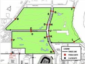
Image 2 & 3: Journal pages.


There were a lot of birds chirping, I heard at least 4 different kinds of birds. One kind were shrikes based on the appearance and sparrows and jays based on the appearance as well. There were trails along the river, few people were taking a walk. There were dragonflies and burrows in the ground around the ponds, showing that there might be rabbits and moles in the grassland. There was a lot of cricket noises along the river and there were few geese swimming on the river as well. More than 5 squirrels were spotted, there were a lot of pine nuts on the floor near the pine trees which the squirrels seemed to be collecting.
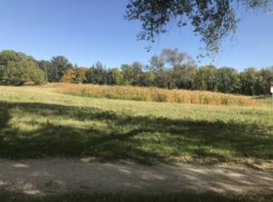
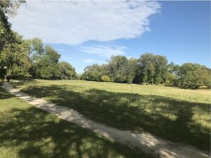
Image 4 & 5: open grass land and trails.
Based on my observations the three questions I asked are:
- How has the geese population affected the role of the other wildlife in this grassland area?
- How does the human activity around the south wood lands affect the deer and geese activity in the open grassland and riverbank area?
- How much resources are available for the urban geese when the migratory geese arrive in the fall? And also how the weather plays a role in how much deer activity is noted?
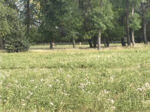 Image 6: Deer feeding on the vegetation.
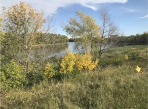 Image 7: The Red River.
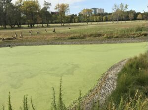 Image 8: Geese around pond 1.
Blog Post 5 – Design Reflections
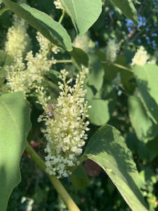
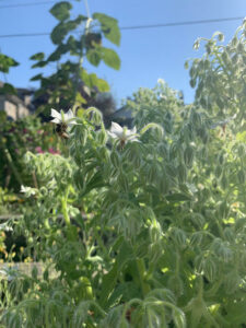
So far I have not had much difficulty in actually implementing my sampling strategy, but I did have some questions to answer before initiating my strategy. Firstly, I had to consider that although I am observing honeybee activity in relation to the road, I had to find plants in each location that would be similar enough to sample the activity of the honeybees. I have chosen 3 plants that all contain flowers and leaves and seem to have honeybee activity regularly.
After doing my replications, I was somewhat surprised with the results! At a quick glance, the elderflower shrub has an extensive amount of insect activity. But after observing the plant for 5 minute increments, I noticed that majority of these insects were not the Western Honeybee. Regardless of this, I was able to obtain some number for each replicate to add to my study.
I think I will continue to collect data using the same technique as it makes the most sense for my study. I will keep the same plants I initially observed as I think they are the most similar and will assist in the accuracy of my study. Not only are these plants similar in looks, but they are also all cultivated plants which will help to keep my samples similar as opposed to having some cultivated plants and some naturally occurring plants.
Below is my replicate chart and the plants I intend on using for my study:
|
Replicate Number |
Time of Point Count |
Number of Western Honeybee Visits |
|
1st |
1259hr |
17 |
|
2nd |
1304hr |
11 |
|
3rd |
1309hr |
9 |
|
4th |
1314hr |
14 |
|
5th |
1319hr |
15 |
Blog Post 9: Field Research Reflections
In reflecting on my experience designing and carrying out my first field experiment there were some aspects I really enjoyed, and others less so. I found a lot of satisfaction in the initial process of going out and closely observing nature. I liked that it embraced the principles of curiosity and the simple appreciation of being outdoors. I didn’t mind the process of picking a topic and designing my study, but I would’ve preferred doing it as part of a team. I believe my learning style is best served by having a team to bounce ideas off of, and particularly for my first field research project, I would’ve benefitted from working directly with someone else in the field. Admittedly, there were moments during the long hours of data collection when I was alone and morale was low.
That being said, I didn’t run into any real issues with the implementation of my project that required major changes, aside from adjusting quadrat sizes, equipment and minor alterations to my hypothesis/predictions, and am really appreciative of the experience. I feel that I have broadened my toolbelt so as to be better prepared for future endeavours in research and have definitely learned a lot regarding all the details that must be considered when developing a sampling strategy. Finally, throughout the data collection process I garnered a strong appreciation for the meticulousness, attention to detail, and patience that is endured in the development of ecological theory.
Blog Post 8: Tables and Graphs
I used a scatter plot to illustrate the relationship between soil moisture and percent slope from the data I collected. I ran into two primary challenges when creating my figure. The first issue I encountered was how to organize it in a way that maintained its clarity. I had 150 data points to plot on the figure, and after inputting them all I felt that the graph looked disorganized and busy, making it difficult to analyze. I tried to rectify this issue by including three extra plot points depicting the mean values across each of my three subareas, as well as trendlines, in an attempt to make patterns throughout the data more easily discernable. Inevitably, I don’t believe this was successful. The second issue I ran into was with my figure caption. I struggled with getting it properly formatted underneath my graph and additionally, I found it difficult to write it in such a way that explained my graph concisely. Word choice was difficult, redundancy as well as clarity were a challenge for me. I need to find a better way to more clearly describe which data was drawn from which subarea.
The data from my research were not totally consistent with my hypothesis. Soil moisture was, in fact, lowest where I thought it would be highest however, trees were largest at the bottom of the hill, as expected. Tree density was also highest at the bottom of the hill however, I predicted it would be highest at the midpoint. In terms of unexpected patterns, it appears that tree species distribution showed some degree of zonation across the slope.
Further research could explore this topic more in depth by measuring soil moisture within deeper layers of soil using more sophisticated tools, and look at changes in soil moisture as it relates to precipitation by collecting data at a variety of dates after a rainstorm to see how runoff might impact near-surface soil moisture across a slope.
Blog Post 4 – Sample Strategies
Below are the results of the 3 sampling strategies used in the virtual forest tutorial:
| Virtual Forest Assignment Table | Sampling Method | ||
| Species | Systematic | Random | Haphazard |
| Eastern Hemlock
True: 469.9 |
Estimated: 408.0
Percentage Error: 13.2% |
Estimated: 508.7
Percentage Error: 8.3% |
Estimated: 388.0
Percentage Error: 17.4% |
| Sweet Birch
True: 117.5 |
Estimated: 92.0
Percentage error: 21.7% |
Estimated: 130.4
Percentage Error: 11.0% |
Estimated: 160.0
Percentage Error: 36.2% |
| Yellow Birch
True: 108.9 |
Estimated: 96.0
Percentage Error: 11.8% |
Estimated: 78.3
Percentage Error: 28.1% |
Estimated: 156.0
Percentage Error: 43.3% |
| Chestnut Oak
True: 87.5 |
Estimated: 124.0
Percentage Error: 41.7% |
Estimated: 108.7
Percentage Error: 24.2% |
Estimated: 100.0
Percentage Error: 14.3% |
| Red Maple
True: 118.9 |
Estimated: 140.0
Percentage error: 17.7% |
Estimated: 126.1
Percentage Error: 6.1% |
Estimated: 108.0
Percentage Error: 9.2% |
| Striped Maple
True: 17.5 |
Estimated: 36.0
Percentage error: 105.7% |
Estimated: 13.0
Percentage Error: 25.7% |
Estimated: 28.0
Percentage Error: 60% |
| White Pine
True: 8.4 |
Estimated: 0.0
Percentage error: 100% |
Estimated: 0.0
Percentage Error: 100% |
Estimated: 8.0
Percentage Error: 4.8% |
- Based on the information provided, the fastest estimated sampling time was the random sampling method estimated at 12 hours and 19 minutes.
- The 2 most common species are the Eastern Hemlock and Sweet Birch. As you can see from the data presented above, the random sampling method yielded the lowest percentage error. For the 2 rarest species – Striped maple and White pine – the random sampling method yielded the lowest percentage error for only 1 of them (Striped maple), whereas the White pine’s lowest percentage error was in the hap hazardous sampling method. The accuracy did seem to change with species abundance generally speaking.
- After taking the mean percentage error of each sampling strategy these were my results – Systematic (44.5%), Random (29.1%) and Hap Hazardous (26.5%). This would be indicative that the Hap Hazardous Sampling Strategy is the most accurate out of all 3 strategies.