Blog Post 1: Observations

The area I have chosen is on private land in a rural farm community outside of Taylor, British Columbia. It is approximately 12 acres in total with a predominately coniferous forest with a ravine that holds a small creek and both sides of the creek are farmed fields. The ravine itself boasts a lot of  value with many different features such as small wetlands due to beaver (Castor canadensis) activity, pooling water and the running creek itself. It is important to note the creek is a lot more bank full than normal due to the increased amount of precipitation.

Figure 1. Area in yellow is the perimeter of the observation site. Red line that was walked within the area.

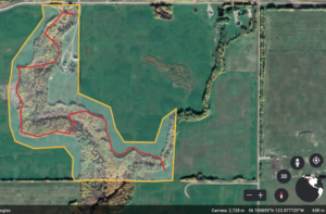
I first visited this area on July 14th, 2020 at 1400 hrs until approximately 1600 hrs. The weather was 20 degrees celsius with some overcast but, it was incredibly muggy. I remained in the area that is highlighted in yellow and scouted around within that perimeter that can be represented in the red line. The size of the chosen observation area is approximately  0.31 square kilometres.

The vegetation from the bottom of the ravine consisted of typical wetter vegetation species such as:

  • Lady fern (Athyrium filix-femina)
  • Meadow Horsetail (Equisetum pratense)

And then carrying up the slope gradient the vegetation has noticeable changes leading into species such as

  • Prickly Wild Rose (Rose acicularis)
  • Cows Parsnip (Heracleum maculatum)
  • A few willow species (Salix spp)
  • Saskatoon (Amelanchier alnofolia) 
  • Soopolallie (Shepherdia canadensis) 

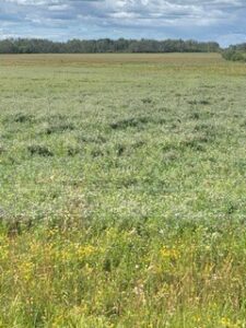
Leaving the ravine and going into the field there are a good mix such as

  • Foxtail Barley (Hordeum jubatum)
  • Timothy (Phleum prantense) 
  • Kentucky Bluegrass (Poa prantensis)
  • Northern Brome (Bromus inermis)
  • Alsike Clover (Trifolium hybridum)
  • Alfalfa (Medicago sativa) 

This crop farmed field is mostly Alfalfa with the other species making random appearances throughout the field. It would be good to do a proper walk though out the field as well.

Figure 2. View of the field that is hayed yearly.

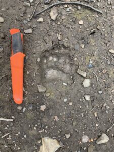
There was also noted to be Black bear activity (Ursus americanus) due to several ant hills being dug up and some old marking in trees as well as tracks.

Figure 3. Black bear tracks located on the south side of the ravine.

There is also a lot of ungulate activity in terms of tracks and droppings. Mostly White tailed deer (Odocoileus virginianus) and Moose (Alces alces). Elk (Cervus canadensis) are also known to frequent the area but, determining the difference in tracks is a little tricky. 

Potential subjects and relevant questions

Question 1: Do the species of ungulates that frequent the upper field selectively graze? (I feel this is where I will go with my study)

Question 2: Despite being older and potentially no longer in use, how much is the old beaver dam impacting the area of the lower ravine?

Question 3: Is this relatively small area able to support a Black bear for a suitable territory or is it a series of areas frequented?


Blog Post 5: Design reflections

I did have some difficulties implementing my strategy. Randomly sampling made it hard to select which plant to measure when they were not as abundant in some areas. As well, trying to get an accurate representation from one plant branch of the plant became very challenging. The data was surprising because the plant heights between the two transects looked very different but ended up being very similar.

I will continue collecting my data with the same sampling method (random) with some changes. My data will be continued to be collected at random but i will measure several branches of each plant to average the height for each sample.

Blog Post 4: Sampling Strategies

% error of area densities for systematic, random and haphazard sampling types in the Synder-Middlesworth Natural Area:

Systematic common species % error:

Eastern Hemlock: 20% error

Sweet Birch: 9.8% error

Systematic rare species % error:

Striped Maple: 18.9%

White Pine: 48.8%

Random common species % error:

Eastern Hemlock: 31.7%

Sweet Birch: 14.9%

Random rare species % error:

Striped Maple: 281.1%

White Pine: 50%

Haphazard common species % error:

Eastern Hemlock: 43.9%

Sweet Birch: 53.2%

Haphazard rare species % error:

Striped Maple: 151.4%

White Pine: 100%

The systematic sampling had the lowest sample time with 12hrs 4mins. It was also the most accurate for both common and rare species. Next was random sampling that would take approximately 12hrs 53mins. The slowest and least accurate was the haphazard sampling method at 13hrs 11mins. The results overall seemed to be more accurate throughout all three sampling techniques in the more abundant species such as Eastern Hemlock and Sweet Birch. As well, the overall most accurate sampling method appears to be the systematic method.

Post 3: Ongoing Field Observations

I plan on studying Arctostaphylos uva-ursi (Kinnikinnick).

Hypothesis: Overhead plant life will negatively effect the height of kinnikinnick.

Prediction: Plant height will decrease under layers of vegetation

Response variable: Kinnikinnick

Explanatory variable: Overhead plant life (continuous)

Study is continuous. (Regression approach)

An underlying process that may have caused the observed patterns could be soil type. The open areas had little to no LFH layer and the soil was coarse and very well-drained. The areas of more cover had a little larger of an LFH layer and the soil was less course but still well-drained. This could be the underlying cause of the pigment and growth difference between the two locations.

blog post 3 journal

Post 2: Sources of Scientific Information

The source is on The Effect of NaCl and CMA on the Growth and Morphology of Arctostaphylos uva-ursi (Kinnikinnick).

Young, J. P., Rallings, A., Rutherford, P. M., & Booth, A. L. (2012, January 12). The Effect of NaCl and CMA on the Growth and Morphology of Arctostaphylos uva-ursi (Kinnikinnick). Retrieved August 09, 2020, from https://www.hindawi.com/journals/jb/2012/789879/

This article is academic peer-reviewed research material. The article is formatted as: Abstract, Information, Materials and Methods, Results, Discussion, Acknowledgments and References. This follows the academic scientific article format. I know this is peer-reviewed because at the beginning of the article it states “Academic Editor: Sergi Munne-Bosch”. It also states “Revised 27 Sep 2011. The article is made clear as a research paper when stating materials and methods. Within that section there is a table showing the treatments used in the experiment and a figure showing portions measured of the plant.

Blog Post #6-Data Collection

I have been collecting data for eight weeks over the course of the summer, to coincide with the mating season of frogs and toads on Prince Edward Island. I had four replicates at five locations randomly chosen throughout the South Shore Watershed of Prince Edward Island.

Every two weeks, I would visit five sites after sunset and record their mating calls with my iphone and I also recorded any visual sightings. Prior to the start of my data collection, I placed water temperature loggers at each site, so I was able to record water temperature for each night I was recording the calls. I did not have any trouble sampling, with the exception of mosquitos that attacked me mercilessly. I haven’t noticed any patterns that necessarily agree or disagree with my hypothesis-It is difficult to determine species abundance, especially at night with frogs. I am concerned that my data will show more correlation with mating season than farming. I have already figured on confounding factors based on their actual breeding patterns. I often find myself in these locations during the day, and I am able to see an abundance of leopard frogs, but I don’t hear them at night when recording. Conversely, I never see Spring Peepers, but I record them in abundance.

Blog Post #5-Design Reflections

I have decided to do an abundance study of frogs and toads of PEI and their distance from active farming sites. We only have four frogs-some will say five, but the pickerel frog hasn’t been seen here since 2003, and one toad. The green frog (Rana clamitans), the wood frog (Rana sylvatica), the leopard frog (Rana pipiens), spring peepers (Pseudacris crucifer), and the American toad (Bufo americanus).

My hypothesis is that the species abundance increases as the distance from active farming increases.

I have chosen five sites at random, however, I had to make sure that they had the right environment to support the frogs and toads, so they are all fresh-water riparian sites. I chose those sites and will be measuring the distance to active farming sites through arcGIS. I had some water chemistry analyzed at each of the five sites, however, I only had the funds for one sample at each site, so, depending on their nitrate and phosphorous levels, I will maybe only use this data in my discussion, to hopefully support my hypotheses.

I will drive to each of the five sites during the breeding season at dusk and record their calls for five minutes with my iPhone, then analyze the recordings using their call to identify them and the Abundance Code for Frogs to determine how many are calling:

0 = no amphibians heard
1 = individuals can be counted (no overlapping calls) – estimate of 1-5 individuals calling at site
2 = calls of individuals are distinguishable, but some calls overlap – estimate of 6-10 individuals calling at
site
3 = full chorus, or continuous calls, where individuals cannot be distinguished – estimate of more than
10 individuals calling at the site.

Frogs only call during mating season, so I intend to do 20 site visits (4 nights, at 5 sites) during this time.


Blog Post 5: Design reflections

In module 3, I collected data for my experiment to understand whether the presence of other plant species (carrots, pumpkins, onions, and peas) have an influence on the growth and abundance of bean plants near (in 30cm distance) them. For the small Assignment #1, I chose one garden plot, to collect my data.

I selected the systematic sampling strategy to record data because it would help me to avoid the experimenter bias while choosing the samples. This also seems like the best approach because it would prevent collecting samples that are clustered in the same area, but instead use the samples that are spread out around the garden bed. The first individual bean plant sample was randomly selected, and then the next samples were systematically selected. From the fifth plant north, then the fifth bean plant East. However, the difficulty with this method was: the garden plot was not large enough for the samples to be  spread out perfectly in fives. This is therefore why I plan to use the same approach, systematic sampling technique, but I will record every third plant instead of the fifth. Individual samples will still be spread out, and I will have the opportunity to record even more samples. Also, instead of collecting just the presence of other plants, I will also record what those plants are to be more detailed. This will increase accuracy, and provide more data for the analysis.

The collected data was somewhat surprising because the results were different from my predictions. I predicted that the closer the bean plant would be from these other plants, the more leaves and flowers it would have, which was not reflected in my data. I started to suspect that my hypothesis might be falsified, but I will not know until I collect more data. This opened my mind to think about possible confounding variables.

Some of the confounding variables that could play a role in the abundance of these bean plants could be the type of soil, moisture levels, type of bean plants and planting dates especially between the different garden beds. I will do more observation, and to avoid these possible confounding variables. An approach I plan to take to avoid these confounding variables is to firstly compare the bean plants within the same garden beds, before I could compare the beans in different garden plots who might not share some of these factors.

Finally, more careful observation will increase certainty of more extensive data to be collected on the next trip. In addition, a more detailed recording of data will provide more meaningful data that will lead to a more accurate conclusion.


Post 6: Data Collection

On August 3rd and 4th i collected the data from the remaining three of my four 10 x 10m sample plots, located along the shoreline of Nita Lake. Each sample plot was a replicate. Starting with Plot 1, i put into practice my now slightly more refined technique for determining elevation, with the series of 1 meter vertical poles and string running horizontally until it meets the slope of the shoreline. In the sub-1 meter elevation zone,  Alnus rubra grew densely and i had trouble counting the individuals without accidentally backtracking and double counting. However, i started flagging each tree as i counted them and walking up and back parallel with the shoreline boundary of the plot, recording the trees as i gradually made my way up the slope until i hit the back line of the plot. This made it much easier to ensure that i had an accurate tree count, without double counting or missing any individuals.

I have noticed that the substrate types in the sub 1 meter elevation zone are uniform across the four plots, which i believe could be a result of frequent flooding and erosion, creating deep, soft and moist soil substrates in the low lying areas. This could potentially compromise the testing of my hypothesis, as Alnus rubra dominance in low lying areas may be influenced by substrate type rather than correlating only with frequency of flood disturbance. However, for this reason i recorded all changes in substrate types throughout the different elevations, so by analyzing the species composition in different substrate types throughout  sample plots i should be distinguish and nullify the influence of substrate type in the flood prone zones.

Blog Post #5

I decided to study vegetation diversity with increasing distance from the creek in my home town. My hypothesis was that proximity from the creek would effect the variety of plant life growing in the area. I predicted that, as distance from the creek increased, the variety of vegetation would also increase. I predicted the heardier plants like the Cows Parsnip and grass would survive closer to the creek because they are typically able to survive in a variety conditions. They can grow in shade or direct sunlight and in damp areas as well as drier areas. Other species, such as the wild rose, needs to have a bit of shade as well as not be in areas that are too damp or too dry.

I focussed on the portion of the walking trail starting at 15th street and ending near the public library because the whole creek would be too large of an area for me to properly sample. I stratified the area by the creek into five different sections (t1-t5) as shown on my map below. I took eleven samples from each section. I used a random number generator app on my phone to determine how far I would have to walk in each section before placing my 1m^2 quadrat and sampling.

I stuggled with collecting my data for the areas closest to the creek as some areas were very steep and difficult to walk on. I was forced to estimate where I would be placing my quadrat from the top of some of the inclines because I couldn’t actually get down the slope to place it.

I counted how many different species types I found in each section:

T1-8

T2-8

T3-12

t4-8

t5-4

I was surprised to see that the first two sections didn’t have a higher number of species than the third. I wondered if this was due to the mowing and spraying the city does near the walking trail. This also could be due to the plants near the trail being in direct sunlight.

I think that my method of sampling is working for the most part. I would like to think of a more accurate way to smaple the areas nearest the creek but have yet to come up with a solution (if anyone has one, please let me know). Also, I will need to take more samples in each section. Some of the rarer species I listed didn’t get sampled even once. I found myslef walking past some common species every time due to random luck with the number generator. Taking more samples would give me a better idea of the diversity and abundance of the species in each transect.