Post 5: Design Reflections

I chose the haphazard sampling strategy because the shorelines of Nita lake varies significantly in vegetation abundance as a result of some particularly steep and rocky areas. In order to determine whether elevation from the waterline (flood prevalence) has a relationship with species composition, I needed to sample areas that had sufficient abundance in vegetation and a gradual enough gradient. The results in my first assignment submission are from Site 2, which is one of four sample plots i chose along the shoreline. I am aware that by subjectively selecting sample sites i run the risk of subconsciously tailoring the results to fit my hypothesis, and neglecting other factors aside from elevation that may have an impact on species composition, such as substrate. I analyzed and recorded the substrates in results, and there appeared to be some correlation between substrate type and species composition, particularly in the higher, less flood vulnerable zones.

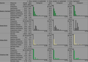
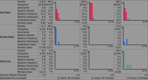
I had predicted that Alnus rubra would be the overwhelmingly dominant species in the sub-2 meter elevation zones, as this would align with my hypothesis that Alnus rubra will be the dominant tree species of flood prone areas on Nita Lake. My results demonstrated this, with Alnus rubra composing 100% of individuals in the sub 1 meter zone and 95% in the 1-2 meter elevation zone. However, i was surprised to see that this trend in species composition continued past the flood prevalent zones, with Alnus rubra comprising 89% of individuals in the 2-3 meter zone. The variable that stood out to me in this zone was substrate, with Alnus rubra only growing in the areas with deeper soil, in contrast to the two Western red cedars growing in a thin layer of soil over large rock slabs. This made me give more consideration to the impact of substrate, as well as flood disturbance, on the distribution of Alnus rubra, and the colonizing behavior of Alnus rubra in non flood disturbed regions.

This sampling exercise was my first attempt at practicing my elevation calculation methods. I lodged an upright pole (using a level) in the mud at the waters edge, with markings from 0cm (at the waterline) up to 1 meter height on the pole. I had a string attached to the pole at the 1m elevation mark that, with a helper, i ran horizontally across to where it met the rising slope of the shore line, and attached it to the ground with a tent peg. I used a level to make the string horizontal. This gave me the 1 meter elevation mark in my sample plot. I then lodged another pole in the ground at the 1 meter mark and went through the same process to make the 2 meter elevation mark. I did this two more times to make the 3 and 4 meter elevation marks. This was a slow and tricky process to begin with, however after finishing the second mark we became much more efficient at it, and i think it provides sufficient accuracy for my purposes. I also used these horizontal string lines to determine the perimeters of my 10 x 10m plot.

I will continue to use the haphazard sampling strategy as i found it to be successful in recording these results.

Post 4: Sampling Strategies

Sampling methods:

I used the area based systematic, area based random, and area based haphazard methods to sample the Snyder-Middlesworth Natural Area.

The area based haphazard method had the fastest sampling time at 12 hours and 28 minutes, followed by area based systematic at 12 hours and 46 minutes, and area based random at 12 hours and 52 minutes.

Percentage error for the two most common species:

Eastern Hemlock

Systematic: 8.1%

Random: 5.1%

Haphazard: 1.6

Red Maple

Systematic: 5.8%

Random: 29.7%

Haphazard: 22.6%


Percentage error for the two rarest species:

Striped Maple

Systematic: 100%

Random: 28.6%

Haphazard: 18.9%

White Pine

Systematic: 90%

Random: 48.8%

Haphazard: 98.8


There appears to be a strong correlation between higher species abundance and higher sampling accuracy, with significantly higher percentage error in the sampling of the rarest species than the sampling of the most common species.

For the two most common species i found the systematic sampling strategy to be the most accurate, while for the two rarest species Random sampling was the most accurate. There appeared to be great variation in the accuracy of the three strategies, and there was no overwhelming stand out in terms of accuracy.


Blog Post #4: Sampling strategies

The three sampling strategies I used in the virtual forest tutorial are Systematic, Random and Haphazard techniques.

I used area based methods to compare among the sample placement strategies. Please find here below, the tables demonstrating the collected sampling data collected on Snyder-Middleswarth Natural Area Community.

Among the three techniques, the Systematic sampling had the fastest estimated sampling time of 12 hours and 36 minutes; whereas Random sampling estimated time was 12 hours, 44 minutes; and 13 hours for the Haphazard sampling method.

Among the two most common species: Eastern Hemlock and Sweet Birch, Haphazard sampling technique was relatively the most accurate giving the lowest percent error of 12.3% for Eastern Hemlock and 25.9% for Sweet Birch.

Random sampling technique gave the lowest percent error for Sweet Birch, 25.5%, which is very close to Haphazard sampling technique; and the second lowest percent error of 16.6% for the Eastern Hemlock species.

In all the three techniques, Systematic sampling seem to be the least accurate due to the highest percent errors in the most common species, 17.4% for Eastern Hemlock, and 28.7% for the Sweet Birch.

The two rarest species appeared to be the Stripped Maple and White Pine. In both Systematic and Random sampling technique the percent error values for the White Pine species is 100% because none of the White Pines were present in the selected samples. Similarly, the percent error is 100% in Stripped Mapple species using the Random sampling technique. However, the percentage error was the lowest, 31.4% in Stripped Maple species using the Haphazard technique; and 60% percent error using the Systemic sampling method. Lastly, the highest percentage error observed was 280% of the White Pine using the Haphazard sampling method.

According to the data above, the overall accuracy is higher in the most common species, and lower in the rarest species in all sampling techniques. So the more abundant the species, the higher the accuracy.

Overall the Haphazard sampling technique was relatively the most accurate of the three techniques.


Blog Post 3: Ongoing Field Observations

Below are the scanned images from my field journal showing the ongoing Field Observations at Duggan Community Garden. This time I decided to narrow my observations to one plant species-the beans (Phaseolus vulgaris)-in the garden.

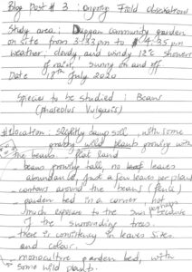
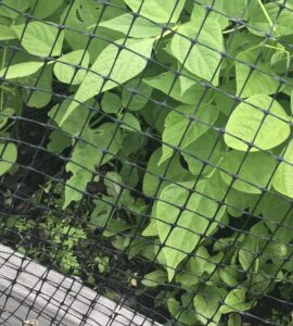
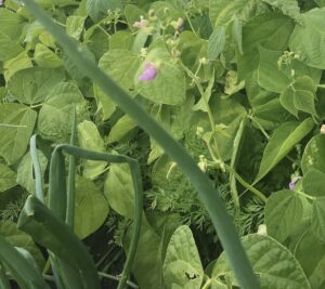
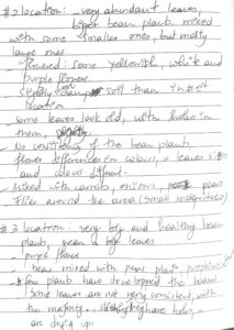
Below are the images of the three locations where I did my observations. Location 1, 2, and 3 respectively.

Processes that may have caused the observed patterns. 

  1. More exposure to the sun may have caused more abundance of the bean plants, especially the larger leaves, and the abundance of flowers.
  2. The presence of other plant species, other than the beans may have induced more growth.

Hypothesis

The growth of bean plants is stimulated by the presence of other plant species in a polyculture environment.

Prediction

The beans in the first location (first garden bed-monoculture) will grow less abundantly (fewer leaves; and fewer flowers per plant) than the beans in the second location (Fifth garden bed from the first one-polyculture).

Variables

Predictor variables: presence or absence of other plant species (in this case carrots, pumpkins, peas and onions) in the same location (one feet) from the bean plants.

Response variable: bean plant abundance (total number of leaves, and flowers per plant)

The response variable is continuous, while the predictor variables is categorical (two level factor).


Blog Post #4

In the virtual forest tutorial, I chose Mohn Mill as my community sample. I chose to do area-based sampling using haphazard, random, and systematic methods. The haphazard method of sampling had the fastest estimated sampling time at 14 hours and 48 minutes, followed by the systematic method (16 hours and 59 minutes), and the random method (18 hours and 13 minutes).

Percentage errors of the two most abundant species:

Red Maple:

  • Haphazard- 2.68%
  • Random- 8.20%
  • Systematic-11.5%

Chestnut Oak:

  • Haphazard-2.90%
  • Random-2.05%
  • Systematic-5.08%

Percentage errors of the two least abundant species:

White Pine:

  • Haphazard- 100%
  • Random- 54.4%
  • Systematic-53.9%

Downy Juneberry:

  • Haphazard-44.0%
  • Random- 53.9%
  • Systematic- 57.0%

It is clear from the data that the more abundant species were more accurate than the less abundant ones. Overall, the random method was most accurate, followed by systematic, and then haphazard. Although haphazard sampling is more time efficient, it is not as accurate as the other two methods. It surprised me to see that haphazard sampling was the most effective for common species and that random/systematic sampling was most effective for uncommon species. I would expect haphazard sampling to be more effective for less common species, as samples are chosen subjectively. I would expect systematic sampling to be most effective for common species. My surprising results are likely due to my not taking enough samples before collecting and analyzing the data or poor choices when choosing quadrants to sample.

Blog Post #3

I have decided to study vegetation abundance with increasing distance from the creek.

  • Cows Parsnip (Heracleum umbellifers)
  • Sweet Clover (Melilotus officinalis)
  • tufted vetch (Vicia cracca)
  • White Clover (Trifolium repens)
  • grasses

I choose four spots along the creek to observe the plants growing there and noticed that wherever the Cows Parsnip was growing, no other plants (besides grass) were growing. The other wildflowers grew everywhere on top of the creek bank, but not near the water. The Cows Parsnip seemed to grow closer to the creek and in damper areas. They also grew more in the shade, while the other wildflowers appeared to grow where there was more sun.


  1. Near Greenhouse.

The wildflowers only grew on the banks of the creeks. The banks here are very steep and the only organism growing near the water is grass. Wildflowers are covering the field next to the walking trail.

2. Near Library.

I stopped seeing the other wildflowers when the Cows Parsnip begins to show up. There is a group of approximately 20 of them in this area. They are in the tall, damp grass and under the shade of the tress. The banks are more shallow here so the other wildflowers are growing closer to the creek.

3. Kin Park Bridge.

The Cows Parsnip are flourishing on the shallow decline to the creek. They are about 2-3 meters from the water.  The closer they get to the creek, the larger and more green they are. The other wildflowers stop near the top of the bank.

4. Across from baseball diamond.

There are tons of Cows Parsnip growing here. There are no other wildflowers here. The Parsnip appears to be greener and have whiter flowers closer to the creek.

It seems as if Cows Parnsip is better suited to survive harsher condition than the other wildflowers. They continue to thrive without sunshine and in very damp areas.

Hypothesis:

My hypothesis is that proximity to the creek will effect the variety of plant life growing in the area.

Prediction:

I predict that the Cows Parsnip will survive closer to the creek due to it being more resiliant to harsh conditions, whereas the vegetation that need more specific conditions (sunlight and water) to survive will not. I predict that the as distance from the creek increases, the variety of plantlife will also increase.

A possible response variable is the presence/absence of the types of vegetation (categorical) and a possible explanatory variable is their distance from the creek/shade of trees (continuous).


Scan of field journal:

Scan (dragged) 2

Scan (dragged)

Blog Post #2

My source of ecological information is on Beaver Assisted River Valley Formation. The link to this scientific source is: https://onlinelibrary.wiley.com/doi/10.1002/rra.1359

This information source is academic peer-reviewed research material. I know that it is an academic source because it is written by experts in the field (writers are affiliated with a university), it includes in-text citations, and has a bibliography. I know that this source is peer-reviewed as the acknowledgements thank Kevin Devito, Jill Johnstone and two other anonymous reviewers for their comments on their early draft. Finally, I know that this is a resource source because it reports the results of a field study (has methods, results, discussion; etc).

Blog Post #1

The area I have chosen to study is in Dawson Creek, BC. I am studying the forest and creek alongside the Dawson Creek walking trail. The creek winds through the walking trail and goes through the city park. My area of study starts near the Dawson Creek Public Library and continues through Kin Park. The Dawson Creek trail follows the creek for about 4.5 kilometres.


My first trip out was on 14/07/2020 at 9:50. It was about 20°C out and sunny. There was a little bit of wind. 

The main area of the creek I focused on was behind the public library. This area is in walking distance of my home, making it a convenient place for me to study.

The creek was low, despite the extreme flooding there was last week. The steeper areas of the creek bank are free of vegetation. All of the plant life on top of the slope is in full bloom.

Observations:

I observed a couple of beaver dams, which led me to wonder what time of the day I was most likely to spot a beaver. I also wondered if they were more likely to chew down certain trees rather than others.  I saw a few tree stumps that had chew marks in them. I also saw a bunch of mud by the creek that had been walked over, but I couldn’t make out any obvious footprints.


Next, I observed some flowers with bumble bees on them, which lead to me wondering whether or not they were more likely to pollinate certain flowers rather than others. I also noticed that the blooming flowers were pointing toward the creek and  I wondered whether or not there was a reason for this. Some flowers/planst I observed were:

  • Prickly Wild Rose (Rose acicularis)
  • Western Aster (Symphyotrichum ascendens)
  • Wild Lupin (Lupinus Perennis)
  • Cows Parsnip (Heracleum maculatum)

I observed some Cows Parsnip by the creek. They became more abundant as I got closer to the creek. I have heard that the sap inside of these can cause burns. The plants I saw and measured were around 58 inches tall.

I could hear lots of birds, but saw very few. Three birds that I saw were the:

  •  Black-billed magpie (Pica hudsonia)
  • Small Brown Bird (Unsure of species)
  • Crow (C. caurinus)

Due to my study area being near the public waking trail and park, there were many signs of human activity. There were plenty of human-made trails that went down to the creek.

Some potential study subjects for my project are:

  • Beavers (Caster canadensis)
  • Bumble bees (Bombus spp.)
  • Giant hogweed (Heracleum mantegazzianum)
  • Black-billed magpie (Pica hudsonia)

Three questions that could possibly help to form the subject of my research project are:

1. Do beavers have a preferred tree species? How is tree selection changed by availability and human activity? What effect do beavers have on the surrounding environment due to their activity? How does flooding effect them?

2. Which wildflowers are bees most likely to pollinate? Is there a specific species or colour that they are more attracted to?

3. Why is there fewer signs of vegetation near the water? It gets slightly less green as you go further down the slope. The giant hogweed, however, becomes more abundant as we near the creak. What is it that makes this species better suited to survive than every other species in the area?

Scan of my field journal:

Scan


Post 3: Ongoing Field Observations

Organism Studied: Alnus rubra (red alder)

Environmental Gradient: The environmental gradient of the study area is the rise in elevation from the shoreline to the railway and the corresponding changes in soil type, drainage and exposure to flood disturbance. Alnus rubra appears to dominate the lower elevations while coniferous species dominate the higher elevations.

I have selected 4 sites along a 100 metre stretch of shoreline. Some parts of the shoreline are very steep and rocky, with limited vegetation. I consequently selected 4 sites that had a more gradual slope, and thus had sufficient vegetation to demonstrate a response to elevation, in regards to species type, abundance and maturity.

Site 1:
Roughly one quarter of the site is a low lying flat area, within 1 metre in vertical elevation from the waterline. The soil is soft, dense and deep, with a layer of leaf and stick detritus completely covering it. It appears that only species present here is alnus rubra, with many young plants covering the area as well as 5 mature trees over approximately 8 metres tall. There are two western red cedars and one western hemlock between 6 and 8 metres tall at the top of the slope, approximately 5 metres above the waterline.

Site 2:
Young alnus rubra plants are growing densely in the area below 2 metres in vertical elevation from the shoreline. The area has deep moist soil covered in leaf and stick matter. The slope rises steeply over large stone boulders. Above 2 metres in elevation, several mature western red cedars (6-12 metres) grow in loose sandy soil on the boulders. At around 5 metres in elevation, several Douglas firs and western red cedars (all over 5m tall), and some young western red cedars are present.

Site 3:
Site 3 rises and dips in several areas, and is mostly lower than 3 metres above the water level. The southern half of the site has a rocky surface with a thin layer of course soil that rises from the shoreline for 5 metres before sloping downwards to an area of thicker moist soils. The higher rocky ground has a several mature (5-15m tall) western red cedars and Douglas fir trees. The northern side of the site is lower lying, covered in grasses, mosses or dead leaf matter, with soft deep, moist soils. There are many smaller red alder plants and 5 mature red alder trees over 6 metres tall.

Site 4:
Most of site 4 is less than 1 metre above the lake water level. These areas have deep moist soils covered either by grasses or leaf detritus. There are many young alnus rubra growing in these low lying areas and 5 mature alnus rubra trees over 5 metres in height. At the top of the slope, approximately 5 metres above the water level are some young western red cedar trees.

In all four sites the low-lying areas appear to be dominated by alnus rubra. These areas are mostly occupied by mosses, grasses and young alnus rubra, and the soils are deep, spongy and moist. The low areas are generally flat, and the land only rises where there are rock formations, which suggests to me that these areas are flood plains that have come about from erosion of softer parts of the shoreline. Walking further north along the shoreline I observed a grass and young red alder covered area beside a creek that was now submerged due to the increased creek flow from spring snow melts. This helped support my idea that these areas are likely subject to flood inundation. The vast majority of the alnus rubra in the low lying areas are young plants less than 50cm tall, which could be related to the frequency of flood disturbances, and red alder possibly being a colonizing species. The rocky, more elevated areas seemed to be dominated by mature conifers. Their age indicates that the area may not have not been subject to a significant flood disturbance for a long time, and the fact that there are no young conifer species at lower elevations might suggest that alnus rubra colonizes these areas before conifers do following floods, they out compete conifers there, or they are more resistant to flood disturbances so conifers are less likely to survive a flood.

I hence made the hypothesis that:
Alnus rubra will be the dominant tree species in flood prone areas of the Nita Lake shoreline.

Formal prediction:
Alnus rubra will be the most common tree species in areas of the riparian zone less than 2 metres in vertical elevation from the current waterline.

Predictor variable: elevation (continuous)

Response variable: abundance of tree species, age/size of trees (continuous)

Blog Post-9

The study of my research project was straightforward, but I did have to slightly modify my experimental design to make my conclusion stronger by collecting more data. I also have to study behaviour of different species of birds in order to relate to the specific habitat , in which I came across some unknown bird species which can be more interesting to study for future studies.