Blog Post 5: Design Reflections

The main difficulty with my sampling strategy was to do with the site locations. Before I began sampling, I went out to the field and used coordinates to document the areas where there were cedar trees (Thuja plicata) and where there were other trees but no cedar trees present. I then listed off all the coordinates and used a random number generator to select five sites of each type to sample. I planned to walk a number of paces (also generated by a random number generator) from the tree closest to where my GPS said I had reached my destination. This location would be slightly different from where I had taken the coordinates due to GPS inaccuracies caused by the forest canopy (Ordonez Galan et al., 2011). However, I did not take into account the level of imprecision, likely also caused by the tree cover. Instead of taking me to a precise destination as it would in an open area, the GPS only took me to about 20 metres away from the endpoint. To get around this, I began counting my paces from the tree closest to when the GPS had the lowest number of metres left to go. 

The surprising part of the data was that the highest value of biomass collected was from a site with Cedar trees. Sample 3 with Cedar trees had a biomass of 580 g/m2. This value was inconsistent with the rest of the data collected from sites with cedar trees and is 28 g/m2 more than the highest value of the samples without cedar trees. I have gone back to this site and suspect that there are some confounding variables at play here. These variables include the amount of sunlight and the topography of the site.

I will be changing my data collection technique to take these confounding variables into account. To do this, I will ensure that the sites I document with coordinates are not in direct sunlight and have relatively constant terrain (no divots where water could pool). I will then continue to use a random number generator to select the sample sites. Another change that I will be making is to begin taking moisture samples alongside the moss samples. I will choose a day to go out and take soil samples from all the sites. Afterwards, I will weigh them, let them dry out and then weigh them again to find the moisture content.

Bibliography:

Ordonez Galan,C., Rodriguez-Perez, J.R., Martinez Torres, J., & Garcia Nieto, P.J., (2011). Analysis of the influence of forest environments on the accuracy of GPS measurements by using genetic algorithms. ScienceDirect, 54(7-8), 1829-1834
Blog Post 5: Design Reflections

The initial data collection in Module 3 was done on a sunny afternoon. The sampling strategy chosen was to randomly choose ferns using random compass directions and random footsteps between 1 to 15. This was done in each of the areas chosen for study: full sun, partial sun, and shade. The data recorded was the number of fronds on the fern and the length of each frond. The fronds were measured with a flexible tape measure, which allowed for me to measure the frond from the very bottom of the stem to the tip of the leaf. The difficulty in my method of data collection was that I realized just how many fronds that ferns have. I ran out of space in my notebook, having planned for only 10 fronds. I immediately changed my technique when I realized that there were a lot of fronds so I sampled the first ten fronds starting with the frond on top closets to me and then going around in a clockwise direction until I reached that first frond again at which point I went to the second level of fronds and I continued in such a manner until I reached 10 fronds. 

I was surprised that the shaded ferns seemed at a glance to have more numerous and longer fronds. I was similarly surprised that the partial sun fronds tended to have fern neighbors in contrast to the ferns in the sun condition. 

As stated above, I had difficulty with the number of ferns and so adjusted my strategy. While I think that there is some bias in this method, I think that using the same method for measuring fronds will limit the bias. I think that this will improve my research as it means that there is a consistent process for measuring fronds. The randomization of selecting ferns appears to have worked, although I needed to be careful on the steep slope on the west side of the ridge and at times would have to repeat the random selection so I did not walk over a cliff. Otherwise, the method appears to be working well.

Post #9 Field Research Reflections

I ultimately really enjoyed this course and the project. I have spent time in conventional as well as online post secondary and while both have their pros and cons, I really miss having the hands on learning experiences and doing things other than reading from a textbook and filling out assignments. It really made all the difference in terms of how I thought about concepts and made connections because having to be out in nature looking for patterns and really observing translated the information into a mode I could easily remember. I also really enjoy academic literature and the number of studies we had to read for this course really gave me an appreciation for coherent academic literature and I really drew on methods I liked to write my own report.

As for the project itself, I learned a lot about what goes into conducting these studies. Most of the data collection and observations were tedious, cold, and the worst of all: involving math. Furthermore, it was very discouraging to get a nonsignificant result and to later learn about multiple reasons why my experiment failed. On the other hand, it was very good for my ego to have failed and I learned a lot more from what went wrong than I think I would have had the experiment rejected the null hypothesis. To add to that, I also really felt proud at the end of my report having written pages and pages of a study I conducted, commenting on data I collected, picking apart methods that I had created and communicating ideas and concepts I had read about and learned. I now know how more to assign variables and evaluate their validity and the importance of doing the abundance of research before you plan the study rather than after.

I already had a deep appreciation and respect for the natural sciences and ecological theory, but this course really gave me a renewed respect for nature and the incredible amounts of intelligence the natural world holds. I think there is a lot to be learned from it that modern day humans don’t always recognize and through learning all of this information, I felt a little put in my place in terms of my role on the planet as a whole. In addition, I think this intelligence and these concepts can be applied to areas of psychology, which is my main area of study. Human minds in their own way are little ecosystems that have a natural covering of different species (genetics), are subject to disturbances (trauma) and invasive species (human influence), and have their own innate tolerance, resilience, and factors that dictate what state they are in.

Overall, I really enjoyed this course and would like to deeply thank Robyn for all of her hard work.

Blog Post 2: Sources of Scientific Information

The chosen information source to evaluate was the paper “Reconnecting Amphibian Habitat through Small Pond Construction and Enhancement, South Okanagan River Valley, British Columbia, Canada.” Written by S.L. Ashpole, C.A. Bishop, and S.D. Murphy.

This source has been classified as Academic peer-reviewed research material. This is justified by meeting the conditions noted below:

Academic:

The paper is written by expert authors affiliated with institutions and government as stated in the article heading (St. Lawrence University, University of Waterloo, Environment and Climate Change Canada) (Ashpole et al., 2018). The material also uses in text citations to other literature and is complete with a bibliography on pages 13-16.

Peer-reviewed:

“Diversity” is a peer reviewed journal as stated on the publishers website (MDPI, n.d.). The paper also mentions additional referees in the “Acknowledgments” section on page 13 (Ashpole et al., 2018).

Research:

The paper reports results of a study completed by the authors, containing both methods and results sections on pages 2 and 6 respectively (Ashpole et al., 2018).

References:

Ashpole, S. L., Bishop, C. A., & Murphy, S. D. (2018). Reconnecting amphibian habitat through small pond construction and enhancement, South Okanagan River Valley, British Columbia, Canada. Diversity, 10(4), 108. https://doi.org/10.3390/d10040108

MDPI. (n.d.). Diversity. https://www.mdpi.com/journal/diversity

Blog Post 1: Observations

On site: 17:00 hours, February 17th 2021

Location: Mission Creek Regional Park

Weather/conditions: 3°c southern winds, light dusting of recent snowfall, late winter conditions with the sun nearly set.

The chosen study area is approximately five square kilometers (paced) within Mission Creek Regional Park in Kelowna, BC. Located west of the Springfield road park entrance, and on the south side of the creek. The area spans north to south from the creek bank to the apex of the upland north-facing slope, crossing a dyke/trail and forested flood plain. The area is bordered by walking trails on the east and west sides. Historically, Mission Creek was narrowed to protect the city and the dykes are now a popular walking path.

Observations:

The creek flows east to west/southwest, and is mostly frozen on the surface after the recent cold snap. Only small pockets of flow remain visible. The creek bank is comprised of riprap leading to a shrub and small deciduous tree riparian zone, meeting with the dyke built parallel to the creek.

The area descends back to creek elevation (several meters) into a forested flood plain/depression zone to the south. This flood plain contains diverse layered vegetation, with dominant shrubs identified as Oregon Grape (Malonia aquifolium) and Common Snowberry (Symphoricarpos albus). The tree population was fascinating, with such a variety of mature growth; Ponderosa pine, Birch, Douglas Maple, Poplar, Alder were identified. A few young evergreens were spotted growing in the midst. Decaying logs and leaves of several species were noted on the forest floor. Transitioning further south into the uplands, the vegetation thins into that of a dry forest consisting of Ponderosa Pine and Grass at the slope apex.

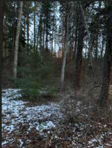
Figure 1: Flood plain looking south towards uplands. (Loverin, 2021)

Questions:

  1.  Is the concentration of deciduous trees in the flood plain related to the creek proximity? or the natural depression of the area?
  2.  Are there fewer Ponderosa Pine closer to the creek? possibly more competition or less favorable conditions?
  3. Does the human disturbance in the area impact the growth and dispersal of the common snowberry (Symphoricarpos albus)?

Field notes – blog post 1

References:

Loverin, K. (2021). Flood plain looking south towards uplands. [photograph].

Parish R., Coupe R., Lloyd D. (1996). Plants of Southern Interior British Columbia. Lone Pine Publishing.

Blog Post 4: Sampling Strategies

Systematic sampling had the fastest sampling time with 12 hours and 6 minutes. This makes sense as the plots used are fairly close together, reducing travel time. Both random sampling and haphazard sampling had estimated sample times around 13 hours, which accounts for their increased distance between plots.


As a species becomes more abundant, the accuracy of the results increases. The average percent error for the most abundant and second most abundant was 11% and 23% respectively. In contrast, the average percent error for the least abundant and the second least abundant was 46% and 113% respectively. This may be because the less abundant species are grouped together so it is much more likely for a plot to have none of that species or a much larger density of that species than its overall density. More abundant species may be more evenly dispersed throughout the study area, resulting in a more accurate representation of them in each plot.


In this scenario, random sampling was the most accurate with an average of 35%. It was also the most consistent in its results without a single result that was extremely high or low. Haphazard sampling got very small percent errors for three of the species, which can not be attributed to anything but luck, since I chose each plot using the “subjectively without preconceived bias” method. The transect used for the systematic sampling did not cross any areas where the two least abundant species were present, which accounts for its high percent errors for those species.

Results: https://photos.app.goo.gl/SgsjpzLhps1ZcRAYA

Blog post 9: Reflections

This was my first time conducting a field research project. As I anticipated, it was quite challenging to conduct field experiments through correspondence studies. With no previous knowledge in research methods, when it came to analyzing and discussing my data, I felt unprepared and lost but I did learn so much and appreciate the process.

My challenges were more based on trying to figure out what I wanted to research and how I was going to develop it. Accumulating the data was easy for me but to analyze it without any background in research methods was where I lacked insight.

From the start, seasonal and climatic variables affected my data collection; it rained most of the summer, and at the peak of vegetation cover, it was difficult to see ant activity. In the spring, I couldn’t identify the vegetation so I decided that I wouldn’t keep track of identifying shrubs, grasses, and trees. I did, however, have a good idea of the general species community of my site.

There was very little research supporting my hypothesis, and that was another challenge. There was no mound in my study which was a bit frustrating because I initially wanted to study correlation of mound presence, soil type and vegetation cover. I soon realized that my topic was quite complex and that ideally this study would be more successful if it was conducted over a longer time frame.


Blog Post 3: Ongoing Observations

For my study, I will be looking at western red cedars (Thuja plicata). For the environmental gradient, I focused on a gradient going from no trees of any species to abundant cedar trees.

The first location had no trees of any species. It was a rocky meadow, where there is very little soil on the surface of the bedrock. The bedrock is mostly covered in a layer of moss that is about 3.7 cm thick  with occasional patches of completely exposed bedrock (see photos for data and species – this data will not be used for my study as the thickness of the moss is dependent on its species but I thought it would be interesting to include it in my description here). The most common moss present was Oligotrichum parallelum. This location had the most moisture of the three locations I observed on the gradient. Water pooled around my feet as I stepped on the moss and there were small puddles in the depressions of the rock.

The second location was on soil with a layer of moss about 6.6 cm thick. The most common species of moss was Kindbergia oregana and there is not a single patch of exposed soil. This location had lots of other low-growing plants, arbutus trees and Douglas fir trees, but no cedar trees. This location was less moist than the last, but still moist enough that my feet would’ve gotten wet if they were not already.

The third location had thinner, more patchy moss and there isn’t a dominant species. There are many sections of exposed soil and lots of debris from fallen branches. I observed 10 living cedar trees from where I was standing and many more that were dead. Moss did not grow at the base of the living cedars but it was much more common at the base of dead cedars. This location was the driest, as it didn’t have as much moss to hold water. My feet would’ve stayed dry if I had stayed in this location!

My hypothesis is “The distribution of Thuja plicata is affected by the biomass of moss present.” and I predict that “Both Thuja plicata and a large amount of moss will not be present in the same location.” The response variable for this study is the presence of cedar trees and the explanatory variable is the biomass of moss. The response variable is categorical and the explanatory variable is continuous.

Link for the photos (I apologize for the slightly blurry parts):

https://photos.app.goo.gl/vAx3R94qfCTjG77w8

Blog Post 2: Sources of Scientific Information

The source I chose is “Plants of Coastal British Columbia including Washington, Oregon and Alaska” which was compiled and edited by Jim Pojar and Andy MacKinnon. I would classify this source as academic, peer-reviewed review material.


It is an academic source because it was written by experts from universities such as the University of Victoria and Simon Fraser University, and the B.C. Forest Service. It includes in-text citations and a bibliography on pages 511 and 512. This source has been “technically reviewed by George Douglas and Chris Marchant” (p. 7), showing that it is peer-reviewed. Finally, this source does not include results from a study so it is review material.


Works cited:

MacKinnon, A., & Pojar, J. (1994). Plants of Coastal British Columbia including Washington, Oregon and Alaska. Lone Pine Publishing.

Blog Post 1: Observations

My study area is about 10 by 10 metres just off of Tannis Way in Nanaimo. The area has three main sections: 

  1. A meadow of exposed conglomerate rock covered by a thin layer of moss and a few small plants that can survive on so little sediment. It also has a footpath where regular human activity has caused vegetation to not grow. This section is on a slant and doesn’t retain water well so the water runs down into muddy pools.
  2. Muddy pools that retain lots of moisture and have collected sediment. These areas are mostly covered in a thick layer of sedge (possibly Carex stylosa but it’s hard to tell since it’s winter) and have few other forms of vegetation.
  3. The last section is under tree cover and has much more diverse vegetation. The trees include Arbutus trees (Arbutus menziesii) and short Douglas firs (Pseudotsuga menziesii).  Underneath the trees is a thick layer of moss, small shrubs like salal (Gaultheria shallon), and low growing plants. Dead trees had lichen and mushrooms growing on them. It is interesting to note that there are no Western Red cedars (Thuja plicata) and the salal is very sparse which is unusual for this area.

This is an Environmentally Protected Area designated by the City of Nanaimo. I visited my study area for the first time on January 21, 2021, at 1611 hours. It is currently winter and that day it was 5°C with a slight breeze and a clear sky.

Some possible questions for my research project: How do the differences in types of moss and thickness of moss affect animal diversity? How do the geographical differences affect plant diversity? What is causing the number of cedars and salal to be less than average?

Photo of the research area and some identified vegetation: https://photos.app.goo.gl/ASLsfzXSEjLjA3RE8

All vegetation was identified using:

MacKinnon, A., & Pojar, J. (1994). Plants of Coastal British Columbia including Washington, Oregon and Alaska. Lone Pine Publishing.