Sampling Strategies

The sampling strategies put a lot into perspective for me. The first strategy of symptomatic sampling was the fastest and seemed to be more accurate than the other sampling strategies, while randomly sampling and subjective sampling took longer and seemed less accurate. Overall, my data suggested it would take 12 hours to gather all this data, which was surprising in general.

Moving onto percentage errors for the two most common species and rarest species was also interesting. Eastern Hemlock and Sweet Birch, the most common species, both had low percentage errors varying from 6% to 15%. When comparing to the Striped Maple and White Pine, both species had percentage errors exceeding 100%. The most accurate sampling strategy for the rare trees and common trees seemed to be random sampling. But overall, for all sampling strategies, the systematic sampling yielded the most accurate results.

I observed that with less species, there was a larger margin for error in sampling, than for the common species. In general, I found I was curious why there are less of Striped Maple and White Pine than the other species of trees.

Overall, a very interesting tutorial!

Post 4: Sampling Strategies

Sampling Strategies

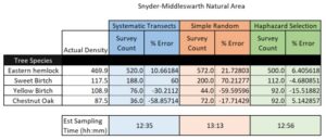
The sampling techniques used in the virtual forest tutorial were the systematic sampling, the random sampling, and haphazard sampling. The technique that had the fastest estimated sample time was the systematic sampling along a topographic gradient at 12 hours and 36 minutes. The random sampling took just a little bit longer at 21 hours and 43 minutes, and the haphazard sampling took the longest at 13 hours and 4 minutes. It is unsurprising that the systematic sampling took the least amount of time as the experimenter would be moving along as transect instead of wandering randomly around.

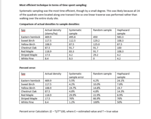
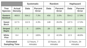
The percent error of the different strategies for the two most common species, Eastern Hemlock and Sweet Birch, and two least common species, the Striped Maple and White Pine, were as follows. The percent error for the Eastern Hemlock was 12.2% for the systematic sampling, 8.2% for the random sampling, and 10.7% for the haphazard sampling. The percent error for the Sweet Birch was 38.7% for the systematic sampling, 29.1% for the random sampling, and 32.8% for the haphazard sampling. The percent error for the Striped Maple was 8.6% for the systematic sampling, 4.6% for the random sampling, and 54.3% for the haphazard sampling. The percent error for the White Pine was 100% for the systematic sampling, 48.8% for the random sampling, and 100% for the haphazard sampling. 

Table 1. Sampling Error (%) for the two most common and two least common species.

Sampling type Eastern Hemlock Sweet Birch Striped Maple White Pine
Systematic Sampling 12.2% 38.7% 8.6% 100%
Random Sampling 8.2% 29.1% 4.6% 48.8%
Haphazard sampling 10.7% 32.8% 54.3% 100%

The accuracy decreased drastically in situations where there were limited species, such as with the White Pine where systematic and haphazard samples had errors of 100%. This was not the case, however, for the Striped Maple where the percent error was very low for the systematic and random sampling, although it was high for the haphazard sampling. The accuracy likely increases with greater abundance as there are more samples and so a greater difference between estimated and actual is needed in contrast to limited samples where the existence or absence of a few samples can change the sampling error.

Overall the four species in Table 1, it appears that random sampling was more accurate than systematic sampling and haphazard sampling. Haphazard sampling was more accurate than systematic sampling where there was a greater population, but had a greater percent error for the Striped Maple and the sample percent error for the White Pine. 

Blog Post 4: Virtual Forest Tutorial

I used the distance-based methods in the virtual forest tutorial.  Systematic sampling was the fastest, taking 4 hours and 15 minutes, random sampling took 4 hours and 38 minutes and haphazard was the slowest at 4 hours and 44 minutes. 

Random sampling had the most accuracy in regards to the two most common tree species and one of the rarer species.  Systematic sampling was the most accurate in regards to the rarest species (white pine).  The haphazard sampling method was not accurate in regards to both abundant and scarce species. 

The systematic sampling technique was more accurate with scarce species than common species and this could be due to the nature of distant-based sampling along one direction.  The systematic sampling method may have not been the most accurate in every species sampled but it did have the most accurate average overall and seems to be a more reliable method of sampling.


Sampling Technique % Error Eastern Hemlock (common) % Error Sweet Birch (common) % White Pine (rare) % Striped Maple (rare)
Systematic 9.9% 64.0% 1.2% 3.4%
Random 3.1% 47.4% 100.0% 0.5%
Haphazard 138.0% 142.9% 142.0% 16.5%

Post 4: Sampling Strategies

Of the three sampling techniques (systematic, random, and haphazard) that I used for the virtual forest tutorial, the technique with the lowest average error rate was the systematic sampling.

The fastest technique was the haphazard sampling (12 hours 34 minutes), but the difference between the fastest and the slowest was only 13 minutes (1.7% of 12 hours 34 minutes), which is fairly negligible.

Screen Shot 2021-02-21 at 22.29.22

Common vs. rare species

The average error rate for the two most common species, Eastern Hemlock and Sweet Birch, was 18.1%. The average error rate for the two least common species, Striped Maple and White Pine, was 42.9%. From this dataset, it appears that the accuracy did decrease with species rarity.

Comparing sampling techniques

Systematic sampling had the lowest average error rate, at 16.7%. Random sampling had the highest average error rate, at 46.2%.

Based on this dataset, systematic sampling appears to be the most efficient and accurate. With systematic sampling, I found the lowest error rates (on average) with only a two-minute time penalty over the fastest technique. The 16% error rate average still seems high, to me, so I would want to re-do this exercise multiple times, probably with more samples, to be able to better identify the technique most efficient in this setting and its most efficient number of samples.

Post 4: Sampling Strategies

There were interesting and unexpected results determined regarding accuracy and time for each method of sampling in this assignment, which was completing the virtual survey of the Snyder-Middleswarth Natural area. The sampling technique which proved to have the fastest time was the systematic transects technique. The sampling style with the lowest percentage of error turned out to be the haphazard selection method. The accuracy of the study was affected by species abundance. The sampling accuracy decreased with a decrease in species abundance. An increase in sampling size would be effective in increasing accuracy. The percentage of error is increased when sample sizes are decreased. I was not necessarily surprised that the systematic technique was the fastest sampling method, but I was somewhat surprised that the haphazard selection method resulted in the lowest percentage of error.

Blog Post 4: Sampling Strategies

Systematic sampling had the fastest sampling time with 12 hours and 6 minutes. This makes sense as the plots used are fairly close together, reducing travel time. Both random sampling and haphazard sampling had estimated sample times around 13 hours, which accounts for their increased distance between plots.


As a species becomes more abundant, the accuracy of the results increases. The average percent error for the most abundant and second most abundant was 11% and 23% respectively. In contrast, the average percent error for the least abundant and the second least abundant was 46% and 113% respectively. This may be because the less abundant species are grouped together so it is much more likely for a plot to have none of that species or a much larger density of that species than its overall density. More abundant species may be more evenly dispersed throughout the study area, resulting in a more accurate representation of them in each plot.


In this scenario, random sampling was the most accurate with an average of 35%. It was also the most consistent in its results without a single result that was extremely high or low. Haphazard sampling got very small percent errors for three of the species, which can not be attributed to anything but luck, since I chose each plot using the “subjectively without preconceived bias” method. The transect used for the systematic sampling did not cross any areas where the two least abundant species were present, which accounts for its high percent errors for those species.

Results: https://photos.app.goo.gl/SgsjpzLhps1ZcRAYA

Post 4: Sampling Strategies

I found the virtual forest tutorial quite interesting. The results were not at all what I expected they would be. The technique with the fastest estimated sampling time was the systematic but I was surprised to see how close all three techniques were. For the two most common species the sampling technique with the lowest percentage of error was the systematic and the highest percentage was the random technique. For the rarest species, the lowest percentage was the random technique and the highest was the systematic. When comparing the three strategy results I noticed that the systematic samples had not picked up any Striped Maple at all. It would seem that the systemic technique may not be the most accurate for the rarer species as it is possible to miss species populations completely. It also makes sense that the systematic system worked so well for the common species. My percentage of error for Sweet Birch was only 1.3%. The species that are common would likely be spread throughout the area being sampled. They would also be present in higher numbers making it more likely that the population will be represented accurately in the samples collected. The systematic technique is not as accurate for rarer species and the random technique was overall the most accurate although not by as much as I had thought prior to this exercise. I think having more sample locations would have increased the accuracy of all the results but especially the results from the less common species. It is too easy to miss the small populations when using small numbers of samples.

Post #4: Sampling Strategies

The Virtual Forests Tutorial revealed results that were surprising in varying degrees. I did the area based tutorial, and I think the most surprising aspect was that there wasn’t a single technique that produced the highest accuracy 100% of the time. While performing the tutorial, I thought that the random sampling method would produce the most accurate results because of the unbiased nature of the design: quadrats were scattered randomly throughout the entire study area as opposed to the single transect line of the systematic design. I assumed the haphazard design would produce the least accurate results (which it generally did), though I attempted to place the haphazard quadrats in spots that seemed “representative” or at least kind of random.

The systematic design had the fastest estimated time at 12 hours 4 minutes, which makes sense as it requires quadrats to be placed along a single line, or bearing. However it wasn’t faster by that much – all three sample designs were estimated to take between 12 and 13 hours.

As far as accuracy was concerned, the most common species encountered had the highest degree of accuracy in abundance estimates, and the accuracy of the estimates was relatively high in both systematic and random sampling placement strategies with random placement marginally the most accurate (except that it did not capture any data on the rarest species); the haphazard placements did not produce accurate abundance estimates for the common species. As a species abundance became scarcer, accuracy went down, except for the capturing of the rarest species (white pine) by the systematic placement of the quadrats, which (out of luck I presume) managed to pick up virtually all of the actual individuals in the sampling area.

Overall, it seemed like the number of samples was adequate to accurately quantify the most common species and would likely be sufficient in a relatively homogenous stand with uniform characteristics, but I would probably want more plots/quadrats if I was striving to capture rare species or a distribution pattern that was more clumped. If I could, I would attempt to use either random or systematic as my sampling placement strategy.

Blog Post 4: Sampling Strategies

After completing the virtual survey of the Snyder-Middleswarth Natural area, there were some interesting observations in regards to the time and accuracy for each sampling method in relation to the population density.

Survey Stats

Fig 1.0 – Survey Stats


OBSERVATIONS REGARDING DATA:

The technique which had the fastest estimated sampling time turned out to be the systemic transects at 12 hours and 35 minutes.

The percentage of error was lowest with the haphazard selection. This was surprising because it allows for inherent bias. When I conducted the virtual selection of survey quadrats, 5 locations were selected in the medial aspect of each topographical section, and spaced equally from west to east. This way a similar sample location was chosen along each topographical feature.
The fact that this was the lowest percentage of error is surprising as I was worried my bias would affect the outcome, but apparently because I applied a system it actually negated an increase in error.

The species abundance also affected accuracy. As the abundance decreased, we saw a decrease in accuracy. The accuracy could likely be improved with an increased sampling size. With any sampling, the lower sample size runs a higher percentage of error.

Overall the haphazard selection appeared to be more accurate than others, but likely due to the systematic bias I introduced by surveying plots equally distanced from one another in an almost grid shaped pattern.


Blog Post 4: Sampling Strategies

For the virtual sampling tutorial, I chose to use area-based sampling for the Snyder-Middleswarth Natural Area. Results are shown in figure 1.

Figure 1: Virtual Sampling Results for 

As shown in the results table, all three sampling methods took over 12 hours to complete, with the random method being the longest at 13 hours and 13 minutes. The two most common species encountered were Eastern Hemlock and Sweet Birch, while the two least encountered (rare) species were Striped Maple and White Pine. Random sampling had the lowest percent error for the Eastern Hemlock, while systematic had the lowest for Sweet Birch. Systematic had a 100% percent error for the two rarest species, Striped Maple and White Pine. Haphazard had the lowest percent error for Striped Maple, while random had the lowest for White Pine, with haphazard only being slightly higher. Systemic generally improved greatly in percent error as species abundance increased. This was also generally true for random sampling as well. Haphazard did not show a consistent trend either way in terms of percent error with a change in species abundance as it greatly improved for the second rarest species but got much worse for the rarest species. For abundant species, I would say that systematic is likely to be the most accurate while haphazard would be the least accurate. For the rare species, systematic is likely to be the least accurate. With 24 sample points, haphazard was able to be quite accurate for Striped Maple but much less accurate for White Pine. This is likely a chance event and I would expect if this was repeated the percent error would be higher for Striped Maple. Likewise, systematic was not very accurate in sampling both rare species in which case increasing the number of sample points would likely improve the degree of accuracy.