Category: Post 8: Tables and Graphs

My figure was relatively easy to put together. It showed the mean number of stems/quadrat counted in each of my treatment areas. As it was a simple comparison between the treatment areas and means, it was not a problem to describe or summarize.

The outcome of the figure was as expected with the calculated values matching what had been visually observed in the field.

The data did give me an idea for further research. The differences in mean values was fairly large and I am wondering if there might be more at play than just mowing frequency that is causing the different growth patterns in the vine.

Overall, I am happy with the outcome of the Figure I created. I initially knew quite quickly what information I wanted to convey, namely soil texture results in relation to slope, however, I struggled with the actual representation of this information. The biggest challenge was deciding how to organize my data in a way that would be discernible to any given audience.

Another challenge, though less so then the data organizing, was the formatting of the caption. Finding the balance of giving enough information without describing things unnecessarily is a practiced skill that I am a rookie at.

Hopefully with time and practice this becomes easier!

I always viewed insects as pests; however, this field research has changed my attitudes towards insects.  The light-trapping technique produces several live specimens hence enabling me to handle and experience live insects.  The insects triggered strong feelings, which were both positive and negative. The feelings were positive because of the shape, colours, and diversity of the insects, while the feelings were negative because of the fear of the bites and diseases. Therefore, educating the importance of insects in the ecosystem using the field experience is very important.  I chose the fieldwork as an important activity in the course of the research project. My project results confirmed that observation and collection of the insects during fieldwork can trigger curiosity and interest in the local natural ecosystems, hence increasing conservation awareness. I did not adequately analyze or evaluate my project’s social advantages because of the small number of participants.

I created a table to show the frequency of conk presence and tree species within the three ecotypes I sampled. I sampled 10 replicates in each ecotype resulting in 120 trees sampled. I wanted to see if the data would show a pattern between tree species, tree health and conk presence. I had some difficulty creating a visual representation of the data as I had originally wanted to show a graph, as I feel they are very clear. However, I had many variables I wanted to compare and I was not able to do this in a clean way with a graph. I was able to show conk frequency per ecotype, tree species frequency per ecotype and average tree health per ecotype. The data is showing support of my claim that conks are opportunistic of trees in poor health, however, I think I would need to increase my sample size to show a stronger argument. It is quite difficult to visually represent what you intend when thinking about the data – the process can leave many things lost in translation.

Given that I am working with data from 10 transects with 11 quadrats each, I had a great deal of trouble organizing my data.  I took field notes in a Google Sheet and used Excel for calculations and data analysis from home.  There were a total of 25 forb species found in the study area and I collected moisture, cover and species abundance data; therefore, (including empty sets) I have 2750 data points (10 x 11 x 25).  It became clear very quickly that naming convention was extremely important when trying to arrange and analyze my data in a meaningful way.  For example: I initially designated my quadrats as T1Q1, T1Q2… T10Q11 (with the number succeeding the “T” being the transect number and the number succeeding the “Q” being the quadrat number).  However, when sorting data alphabetically, T10Q11 would be arranged between T1Q11 and T2Q1.  Therefore, I had to go back and change my naming convention to T01Q01, T01Q2 etc.  This seems like a simple thing, but it caused me a great deal of trouble and illustrated the importance of having “data management-friendly” naming conventions.  I will note that this is, certainly, not the only time I needed to go through and “clean” my data in order to facilitated organizing it in a logical way.

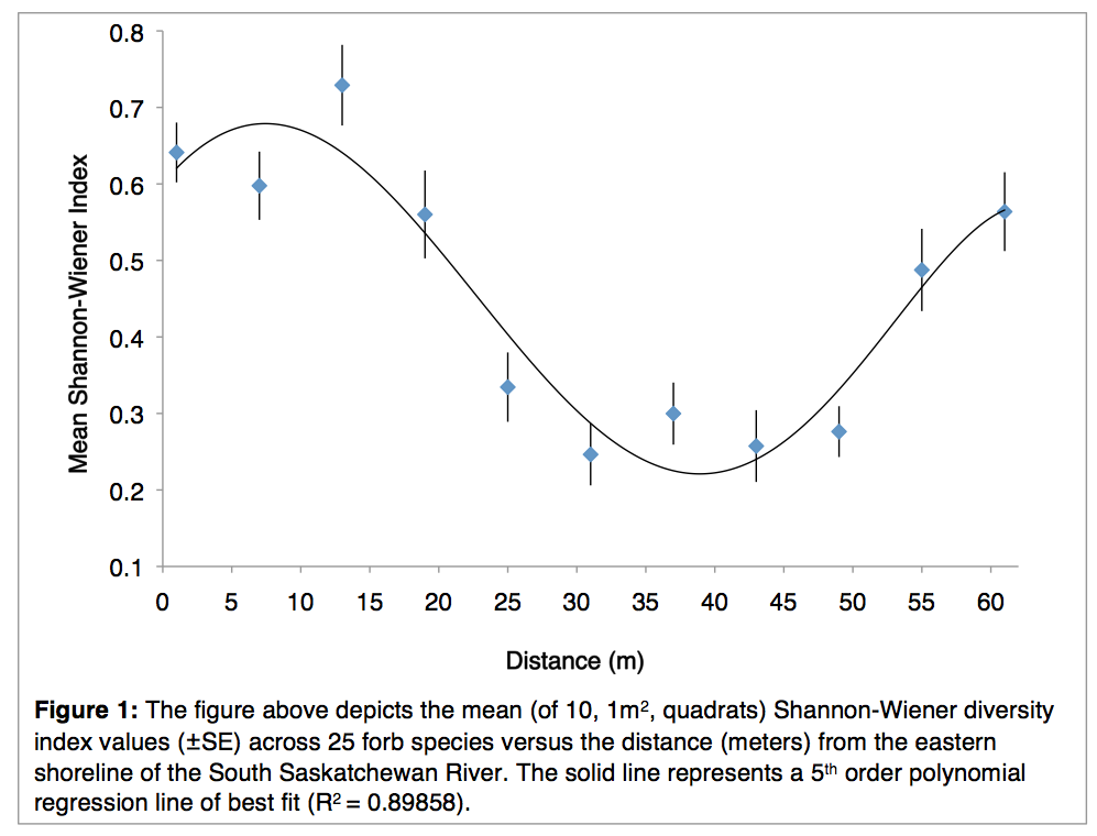
Concerning presenting my data: I struggled to find a singular figure that would readily summarize the overall trends in my project without being convoluted or confusing.  Therefore, I decided to submit a singular graph of the the Shannon-Wiener Index against distance (from the shoreline of the South Saskatchewan River).  I will also note that I did perform calculations for Simpson’s diversity index but have only included the Shannon-Wiener in my submission to avoid ambiguity.

I expected that forb species diversity would be highest at an intermediate area between the extreme ends (the shoreline and the uplands) of the riparian environment I was studying.  While this is true (Figure 1), I was not expecting that the highest level of diversity would occur that close to the shore.  In addition, I was not expecting that forb diversity would be so high approaching the uplands.  While not pictured in this graph (again, for the purpose of keeping it understandable), soil moisture steadily declines and elevation increases as distance increases.  But soil moisture, alone, does not account for the low diversity found from 25-50 m.  Fortunately, I’ve also collected data regarding shrub cover (that I suspect limits forb species).  I also have elevation data from each quadrat and am thinking about using it to calculate the steepness of slope gradient.  As I was sampling my transects, I noticed that both of these factors seemed to relate to quadrats in which no forb species were found.

Regardless, I still have some statistical analyses to perform in order to know which results are significant.