I was happy to do this research study because reading about peatlands and being out in the field built on the interest and appreciation that I already had for them. I think that this is something I will continue to read up on. I had a hard time landing on a design and hypothesis but when I finalized my idea it was fun to execute.
If I were to do this study topic again I would want to do it in the spring or summer. It was very hard to identify plants in the winter and took much longer than I think it would have if there were flowers present.
Engaging in this study has altered my view of ecological theory development. I think my final study was void of biases but I definitely struggled to design a study that didn’t feed into my preconceived notions. I think developing theories in ecology is interesting because of how complicated the real world application is. There are so many things to account for that could influence what you are observing. I learned about so many more ecological interactions in my study than I noticed in my original observations.
The study I am doing seeks to investigate the effect of soil pH on plant diversity in peatlands but it also investigates the connection between soil pH and plant diversity of peatlands to land-use changes. Some of the processes that could be at play in this study are water-logging and soil composition. It could be that the plants that are growing closer to the pathway are not able to grow further into the peatland due to water-logging or soil composition. It might be that the soil that was brought in to build the pathway created a better environment for these specific plants or perhaps the soil that was brought in even carried some viable seeds with it.
The keywords that I would use to summarize my research would be peatland land-use changes, plant diversity and soil pH.
Seasonality and Weather: late winter/early spring 10 degrees. Sunny with relatively clear skies
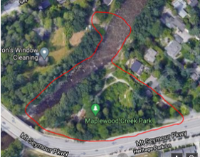
Figure. 1 satellite view of selected observation area showing the northern, eastern, and western entrances. Elevation increases from east to west
The area I have selected to observe is a small, forested area that is slightly elevated and about 223 meters long.
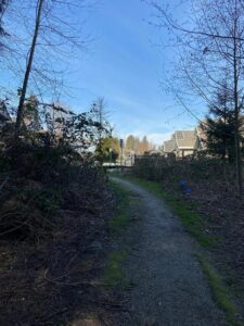
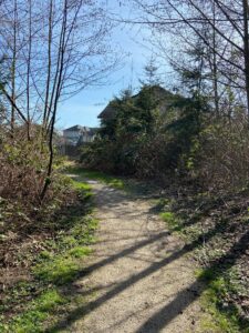
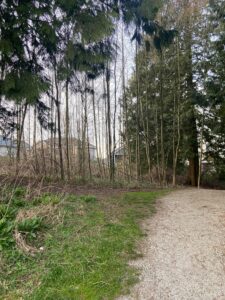
The area is fenced off from residential housing, and the perimeter is mostly surrounded by dried shrubbery and immature trees. There are three entrances to the trail, each having distinctly different vegetation. The northern entrance is bordered by winter killed blackberry bushes, while the eastern entrance is bordered by shrubs consisting of lobed shaped leaves, vines, and few blackberry bushes. The western entrance is surrounded mostly by slender leafless trees with few deciduous trees. The center of the trail is heavily covered by deciduous trees, a lot of which have curved trunks and branches. Moss, lichen, and ferns are found growing in the middle of the trail, and more appear as elevation increases. Moss and lichen seem more prominent growing on the trees found at center of the trail rather than outward. Ferns are found sporadically around the area, although more are found growing in clusters around shaded areas.
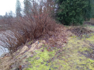
Figure 2. Northern entrance of walking trail.
figure 2. Eastern entrance to trail.
Figure 3. Western entrance to trail.
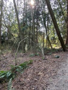
Figure 4. South West of trail showing the irregularity at which trees grow upright and the sporadic growth of ferns.
Based off my observations, the questions I have come up with are as follows:
How do man-made borders affect the density of tree growth in the area and what kind of factors favor a higher density?
How does accessibility/inaccessibility to sunlight affect the sporadic growth of ferns in this area?
How does slope instability affect the curved shape trunks of trees?
The initial data collection in Module 3 was done on a sunny afternoon. The sampling strategy chosen was to randomly choose ferns using random compass directions and random footsteps between 1 to 15. This was done in each of the areas chosen for study: full sun, partial sun, and shade. The data recorded was the number of fronds on the fern and the length of each frond. The fronds were measured with a flexible tape measure, which allowed for me to measure the frond from the very bottom of the stem to the tip of the leaf. The difficulty in my method of data collection was that I realized just how many fronds that ferns have. I ran out of space in my notebook, having planned for only 10 fronds. I immediately changed my technique when I realized that there were a lot of fronds so I sampled the first ten fronds starting with the frond on top closets to me and then going around in a clockwise direction until I reached that first frond again at which point I went to the second level of fronds and I continued in such a manner until I reached 10 fronds.
I was surprised that the shaded ferns seemed at a glance to have more numerous and longer fronds. I was similarly surprised that the partial sun fronds tended to have fern neighbors in contrast to the ferns in the sun condition.
As stated above, I had difficulty with the number of ferns and so adjusted my strategy. While I think that there is some bias in this method, I think that using the same method for measuring fronds will limit the bias. I think that this will improve my research as it means that there is a consistent process for measuring fronds. The randomization of selecting ferns appears to have worked, although I needed to be careful on the steep slope on the west side of the ridge and at times would have to repeat the random selection so I did not walk over a cliff. Otherwise, the method appears to be working well.
Date: Feb 28, 2021 (Winter)
Time: 1400
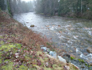
Location: Seymour River/Maplewood Creek Park
Topography: northern cliff is approximately 60 degree slope down to the river, artificially-placed rocks along slope and river bank. Southern slope (park-side) is around 45 degrees with similar rocks like the northern slope.
Weather conditions: Cloudy, slight breeze, approximately 5 degrees Celsius.
Vegetation: forested with native and ornamental trees/shrubs, different species of moss along river bank and upper slope.
Questions:
1. What different types of mosses exist on both sides of the river, where do they grow, and what populations do they support?
2. There is a large growth of invasive Japanese Knotweed on the northern, upper slope of the riverbank. What is currently being done about the species and how has the plant/treatment affected the local ecosystem?
3. What kinds of animals use the park, and what factors attract them to the park?
Location: Kenna Cartwright Park Date: Jan 23, 2021 Time 2:30 pm
10 random numbers between 0 and 1000 were generated on an online random number generator. These figures were used as the distance from the entrance point.
At the park, the distances were measured using a distance measuring phone app (Runkeeper).
At each of the 10 distances, the Ponderosa pine trees in a 5m radius from the point were considered. Only the trees on the upward slope (towards the top of the hill) were considered.
For the pine trees in the radius, the following were recorded: the distance from the entrance point, the elevation and the diameter of the trunk at breast height (DBH) (1.4m). This was repeated for all 10 replicates.
There were no significant problems faced when collecting the measurements for the trees.
An ancillary pattern observed was the increase in DBH with increasing elevation, which increases with the distance from the entry point.
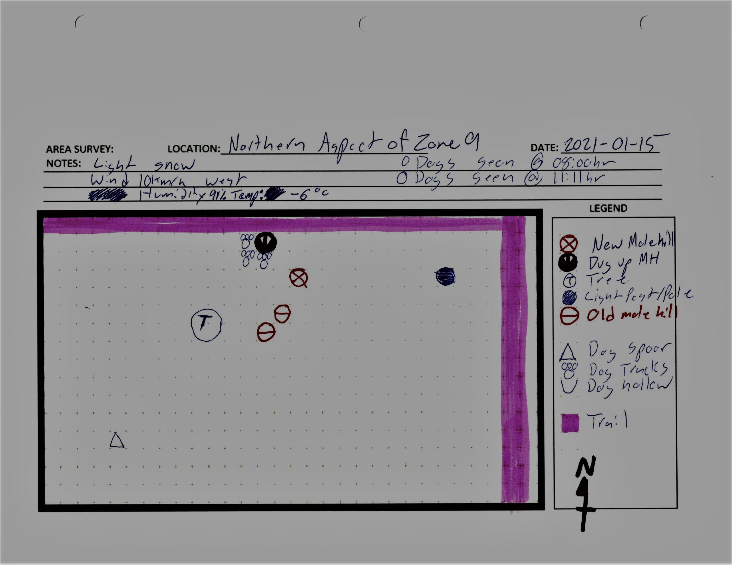
Previously I had been gathering raw data on mole hill activity and predator signs in a 1km x 1km area in western Ukraine. This area was divided into zones each with distinct boundaries and each with a mole colony. The northern half of the area has increased feral canine and stray cat activity.
The intent is to use the data to determine its effect on my null hypothesis, “The number of predators in a given area does not affect the activity of mole colonies in the same area.”
Initially I was using a haphazard sampling technique but had to refine it in order to capture moving pr
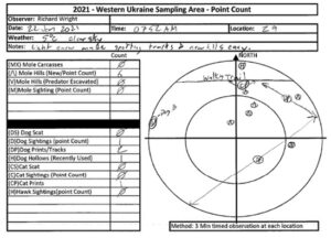
Fig 1. Example of Original Zone observations
edators. The original sampling technique worked well to capture mole activity via the count of new mounds, but failed to be consistent in how predators were recorded. The initial counts were also difficult to conduct because of the duration I was spending at each of the approx. 12 zones. This took most of the morning each day since I was gathering a large amount of spacial data. The time expenditure was significant. There was additional difficulty as I needed to gather data along a chronological gradient. Since the activity of the predators appeared to ebb and flow I also realized that this would need more than a single day of data gathering to do a comparison.
I wanted to capture statistically relevant data, so that I could determine if there was a correlation between these two data points. My solution was to pivot and use a point count with a 3 minute waiting period before moving on to the next location on the route.
This method would be more beneficial as the time frame would give me an opportunity to not only be consiste
Fig 2. New point count method of sampling.
nt in the time of recordings, but also expedite my data collection.
After doing this I graphed some of my data and was surprised that there may (initially) be a correlation between canine predator activity and mole hill activity.
Continuing forward, I will collect data using the point count system. My hope is to do a week or two of data collection each morning to capture both the fluctuations in mole and predator activity. This alteration in data collection should improve consistent precision in my data gathering while reducing time spent.
I am looking forward to collating all of the data and seeing the results.
Originally, the sampling method selected was the belt transect and the trees that were being studied were both the ponderosa pine and douglas fir. The trees were counted in 50×10 m transects. Only the trees on the upward slope (going towards the top of the hill) were counted due to the scarce evergreen tree cover on the downward slopes. The belt transects were the sampling units and they were collected at 10 random distances in the 1000m from the entrance to the park. This sampling method was too broad and did not take into account other factors; data obtained would incomplete.
The revised sampling method still involved 10 replicates over the 1000m distance from the entrance point. Only the Ponderosa pine trees were observed in this method. At the sampling points, trees in the 5m radius of the point were observed and the average diameter at breast height (DBH) was determined. Only the trees that are on the upward slope were considered. The distance from the entrance, the average DBH, the highest DBH and the elevation were recorded.
The change in the approach enables analysis of the relationship between anthropogenic activity and the stability of the environment for tree growth while taking into account other factors in the environment.
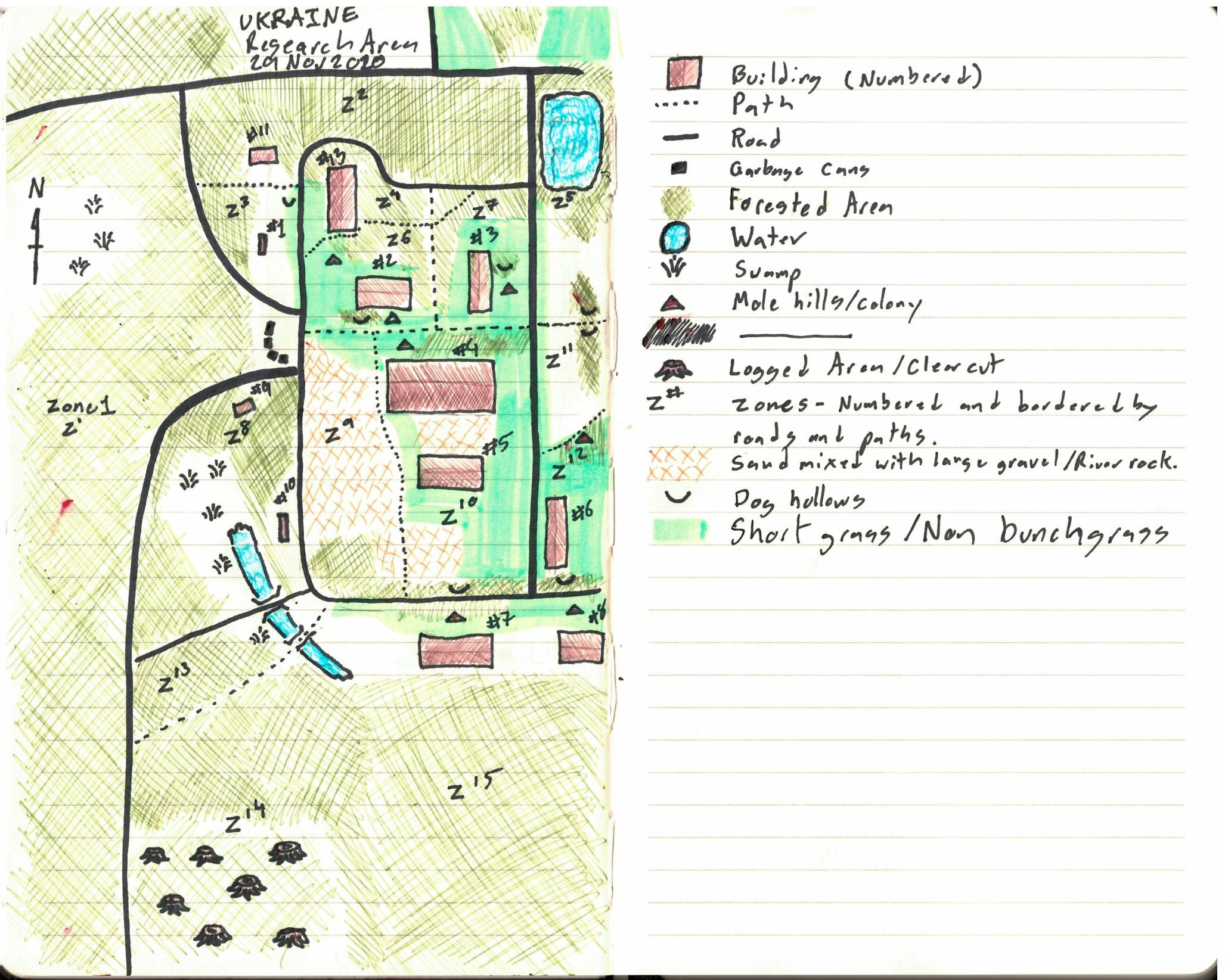
For the course project I have been gathering data on the ecology and communities of a 1km x 1km area in western Ukraine. The following information contains both my ongoing field observations and my considerations regarding a possible hypothesis.
Organism or Biological Attribute:
For the course project I have chosen to study the Eastern European Mole, and how it interacts with local predators such as dogs and cats.
Documentation:
I have been observing and documenting mole colonies, dog sightings, cat sightings, weather conditions, and mole hill activity over the last month in the observation areas. Specifically Zone 9, Zone 15, Zone 12, and zone 7. Contrasting to this, there is a single Zone I have been documenting called ‘Control zone’ east of the observation area which has no Canine or Cat activity observed.
Example of Zone observations
Gradients Observed:
TOPOGRAPHY: In the control area, there is a gradient of topography with approximately a linear grade from the southern aspect dropping approximately 12 feet to the northern most aspect. Of note there is approximately an 8 foot gully near creek on western aspect of observation area.
VEGITATION: The general area which the moles are observed is the grassed areas which sit on a sandy aggregate soil.
PREDATORY CONCENTRATION: There appears to be a higher concentration of predators in north western aspect of observation areas, but less in south eastern area either due to topography, territorial behavior, access to food, or a combination there of.
GROUND: Keeping in mind soil types change throughout the area. Again, the mole hills appear in sandy soil but the depth gradient of tunnels is not able to be directly observed despite the research on moles that indicates that these can go as deep as 6 feet. There is a carpet of decomposing leaves and rich soil under the oak trees (often thick with acorns) but little to none under pine trees.
TEMPORAL: Over time the count of active mole hills, spoor, coil conditions, and weather changes which may affect activity levels of all organisms in observation area.
Three locations inside the Observation area are:
——————————–
North west aspect of Zone 9 – Medium to low dog activity in area/transit point no sleeping
Northwestern Aspect of Zone 15 – Low dog activity in area as they adhere to eastern aspect for midday sleeping.
South eastern aspect of Zone 7 – High Dog activity due to transit+sleeping area
Central area of Zone 12 – Low mole hill count, high dog activity during midday.
Control area: Zero dog/cat activity – Zone A (east of map)
Area of Observation
Processes and Patterns
Anecdotally the mole hills appear more populus and active in zone 9 and 15, as well as the control area to the east. This seems to be inverse to the dog activity in those areas. The temperature changes over time seem to affect the mole activity to some extent.
Hypothesis
The number of predatory dogs and cats in the area directly effects the activity of the colonies in the observation area.
Response variable(continuous): Mole hills along the gradient of dog activity.
Explanatory/Predictor variable (continuous): Number of dogs in the area (based on sightings and new signs)
Initially this appears that a study for this hypothesis would be of a regression design
For the virtual tree sampling tutorial, I selected Mohn Mill. The three sampling strategies used were the Area haphazard method, the distance-haphazard method and the distance random/systematic method. The distance-haphazard method had the fastest sampling time.
The two most common species were Eastern Hemlock and Sweet Birch, and the two rarest species were the Stripped maple and White pine.
The haphazard area method had the lowest percentage error, while the haphazard distance error had the highest percentage error when used to measure the most common species.
For the rare species, the distance random/systematic method had the lowest percentage error, but no Stripped maple trees were located. The haphazard method had the highest percentage error.
The accuracy appeared to be decreasing with a decrease in species abundance for the haphazard methods. However, for the distance random/systematic method, the accuracy increased with decreasing species abundance.