My initial data collection was not difficult. The plot locations were easy to get to other than the 20cm of snow that was unpleasant, but otherwise the terrain is very accessible. The data collected showed that there were actually very few regenerating cottonwood stems, which at first glance, I thought there would be substantially more. There were also less coniferous species found than expected, but this could also be due to the fact that small stems are under the snow, or have been browsed. The amount of woody shrub cover can make plots difficult, as there are a lot of plants to maneuver around. The only modification I may make is increasing plot size from a 3.99 meter radius (50 meters squared) to a 5.64 meter radius (100 meters squared). This could improve the accuracy of the estimated density of tree species, as a larger plot may pick up more species, improving the estimated density. It may also be helpful to actually count the number of shrub species in the plot as opposed to estimating their percent (%) cover, as these plants could be the main reason as to why there are very few coniferous species establishing in the area.
Category: Uncategorized
Blog Post 1: Observations
The study area I have chosen is Central Park on Denman Island, BC, Canada. Central Park is located in approximately the middle of the Island. Central Park is ~147 acres in size and contains two large wetlands and a recovering forest after years of logging in the area. It was logged by horses in 1998 and then heavily logged in the year 2000. The forest is specifically a Coastal Douglas-fir. This kind of forest is relatively rare in B.C. and is threatened. Local conservationists have identified up to 64 different birds that have been spotted in this park.
I visited this area first on June 24th, 2019 between 6:28 and 7:37 PM. On this day the weather was observed to have a low of 12 degrees C and a high of 19 degrees. It was sunny with clouds.
While on this walk I noticed 3 interesting potential study areas with the local ecology:
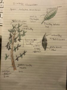
1.) Some but not all arbutus trees appeared to be dying or suffering from some ailment. Some trees had dark covered bark and leaves, while others had very little or no sign of damage. Arbutus are known to shed leafs and bark at various times in the year, but my observations were outside the normal leaf shedding. Why were some of these arbutus trees affected but not others, and why were some of them dying?
2.) In some areas ovate shaped leaves appeared covered in small holes. What organism or local weather or climate caused these holes in these particular areas?
3.) In some areas of the forest and meadows, there appeared to be large concentrations of thistle plants (dozens in a small parcel of land). Why were there so many thistle species in such a small area?
Field Observations:
Blog Post 4: Sampling Strategies
The three sampling strategies I used in the virtual forest were, Distance-systematic, Distance-random, and Distance-haphazard. The results from the three strategies were similar in that species percentages remained in order, and no strategy sampled any White Pine.
Of the three strategies I used, Distance-systematic had the fastest estimated sampling time at 4hrs 16min, followed by Distance-random at 4hrs 30min. The slowest estimated sampling time belonged to the Distance-haphazard strategy, at 4 hrs 49min.
Species:
Eastern Hemlock(EH), Yellow Birch(YB),Striped Maple(SM), White Pine(WP)
%Error/Strategy:
Systematic: EH:15.06%, YB: 97.33%, SM: 17.14%, WP: 100%
Random: EH: 0.17%, YB 1.56%, SM: 56.01%, WP: 100%
Haphazard: EH: 1.92%, YB: 35.45%, SM: 5.14%, WP: 100%
As can be seen, the accuracy varied between species abundance in the different sampling strategies. As per my virtual forest survey, it can be assumed that species does not affect accuracy. The only consistent % error was with White Pine, which was not sampled in any of the three strategies I used, and therefore had a % error of 100%.
The least accurate of the strategies was Distance-systematic, while the other two were fairly similar in their accuracy.
Post 6: Data Collection
My original hypothesis stated that the abundance of dandelions in the centre field of General Brock Park in Vancouver, BC was dependent on their proximity to areas of human activity.
I recently went to do some observations but the dandelions were gone, leading me to modify my hypothesis. I counted the abundance of English daisies (Bellis perennis) as well as other flowers instead.
With the help of my brother, I counted the number of English daisies, red clovers, white clovers, and dandelions in five 1m x 1m quadrats placed randomly in General Brock Park. I did not have any problems implementing my sampling design.
Blog Post 4: Sampling Strategies
Which technique had the fastest estimated sampling time?: Haphazard was the fastest.
Further thoughts: It may also be that with a right hand skew, plus less diffuse error distribution in the haphazard model may actually be a fat tail. If this is the case, then some very important outliers could be hiding in that tail. On second thought, I don’t think I’d want to use this sampling technique where missing the effects of outlying, or phenomenon could have a major impact on stake holders involved in decision making. I wouldn’t use this in helping with ecological assessments around environmental safety, conservation issues regarding extremely endangered species, or economically and culturally vital species, such as salmon or herring populations. If there is error, the randomized model seems represents it more effectively, with a more dispersed deviation around the mean, there by prevent the right skew kurtosis.
Was one sampling strategy more accurate than another? I believe so. I think random sampling shows a more accurate distribution of the deviation. However, haphazard is faster, and easier. If the errors in haphazard are predictable, and can accounted for, it may still be appropriate under certain circumstances.
Blog Post 3: Ongoing Field Observations
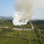
My third blog post comes with a bit of a delay, fortunate I did take notes on the last day of observations, as well as taking photographs of the evidence of the bog fire from last year.
Before proceeding, I’d like to direct the reader’s attention to an article from last year that reported on this fire, and it’s location. I would like to do this in order to provide verification of the bog fire, the time and location at which occured.
Year in review: Bog fire burned: Richmond’s wildfire was one of the biggest blazes in local history.
From the article:
“The summer of 2018 was one of the hottest ever recorded in B.C. and Friday, July 27 is a day that will live long in the memory of Richmond’s fire department.
Early morning reports of smoke coming out of the peat woodland at the DND Lands, near Westminster Highway and Shell Road, quickly developed into a wildfire.” (Campbell, 2018).
I’ve also been trying to determine how to demonstrate to the readers, here, that the burnt over areas I plan on sampling in did indeed experience that same fire a year ago. It occurred to me that in response to their canopies being destroyed by the fire, many of the invasive blueberry, Vaccinium corymbosum, would probably have begun to re-sprout this year. The new vegetative growth, if it was only from this years growth, should not have had time to lignify, so if I observe an abundance of such growth (all green, with no lignified, woody tissues present) then this should be a demonstrable indicator of a fire having occurred within the area of observation in the season prior(summer 2018) to this year’s growing season (2019).
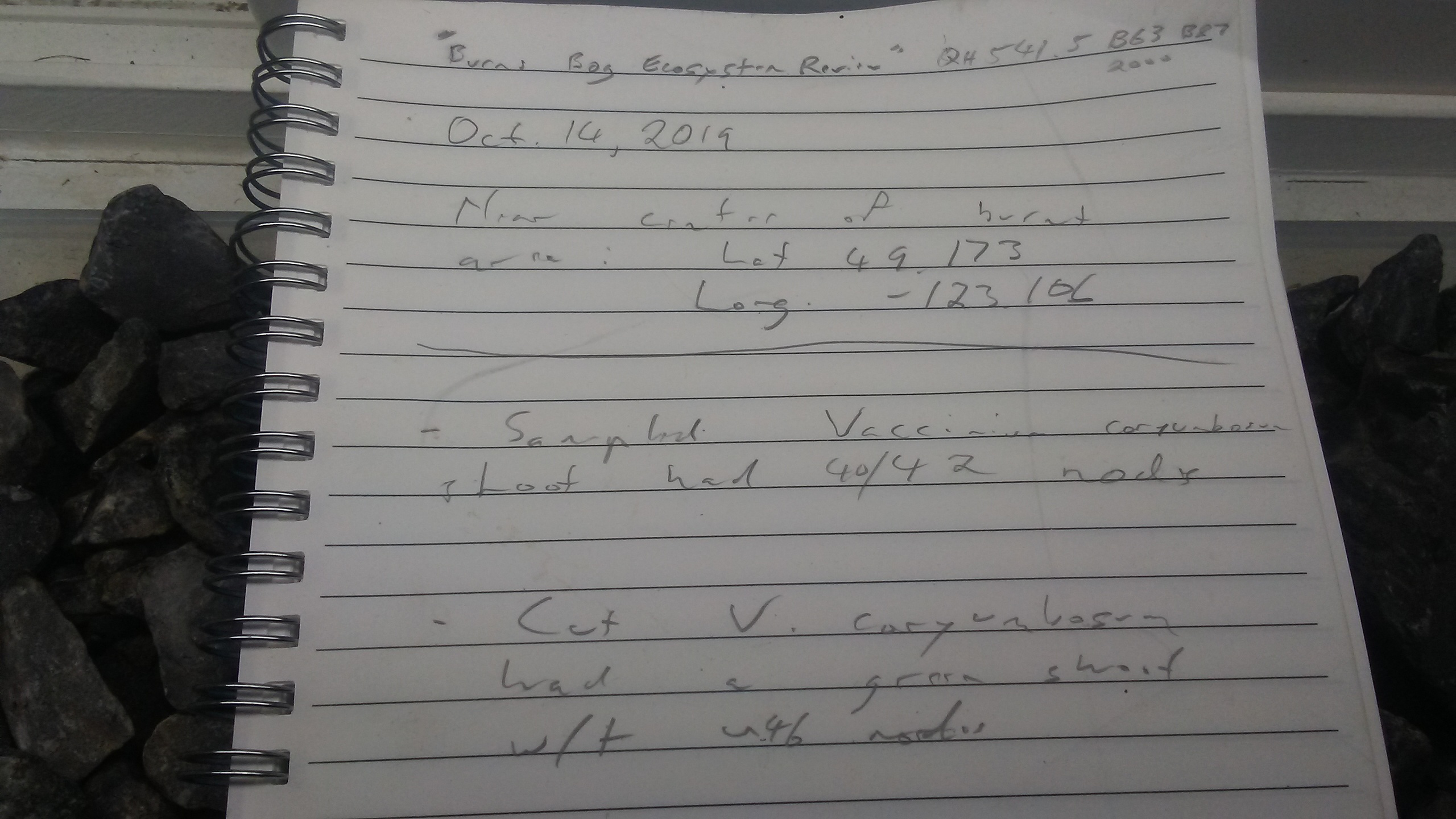
So I returned to the bog at the DND Lands on October 14th, 2019, and made some observations. According to the time stamp in my photos, the time was 5:35pm. Through out the areas that still had residual suit and char, many V. corymbosum plants, who’s canopies had been destroyed, but who’s crowns had not been damaged, showed obvious signs of vigorous greens growth, little to none of which had lignified, or only had very little newly lignified tissue at the bases of the new stems. I also took photographs of this growth, to show that there could only have been a single season’s growth since the last fire, and that fire must have occurred in the areas I will be making my observations.
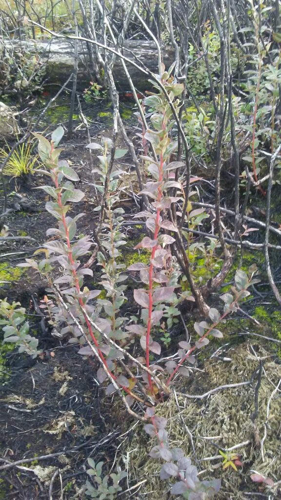
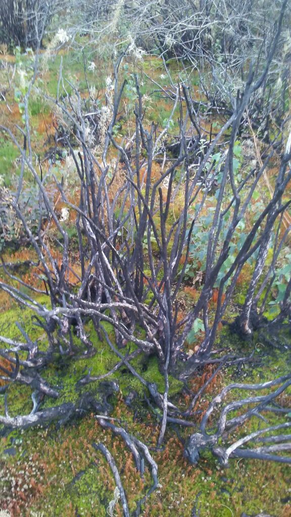
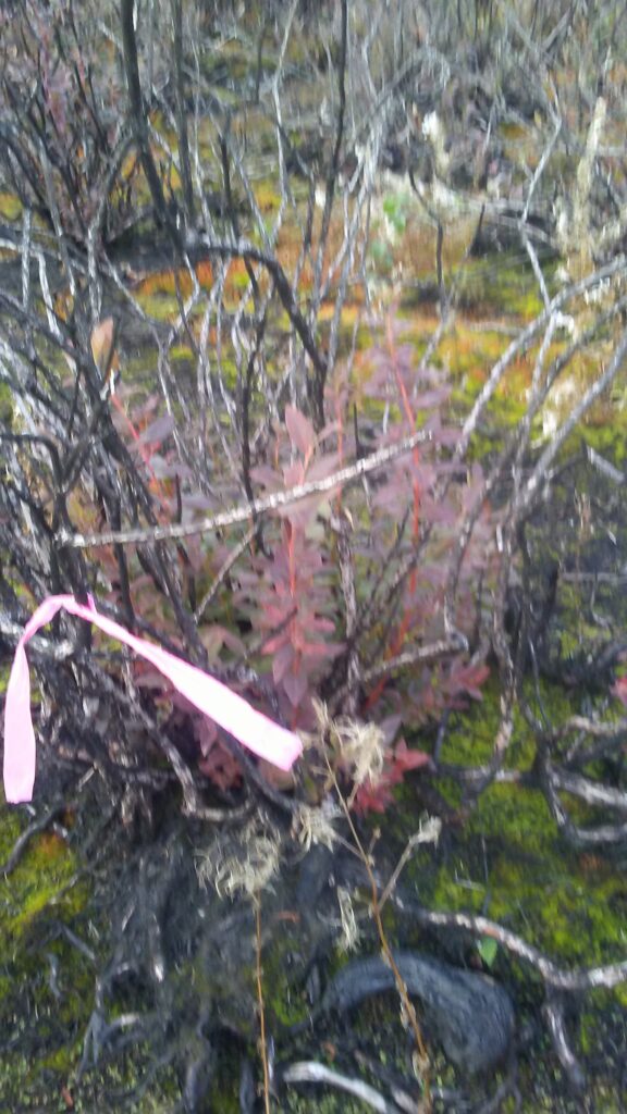
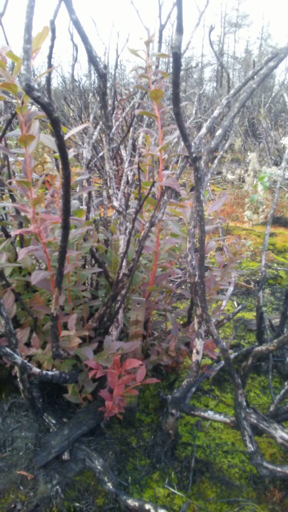
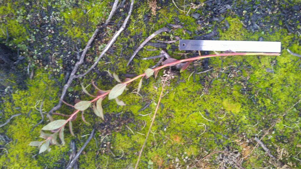
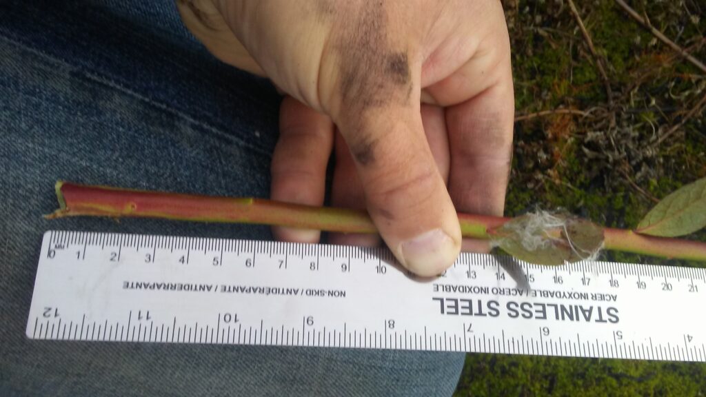
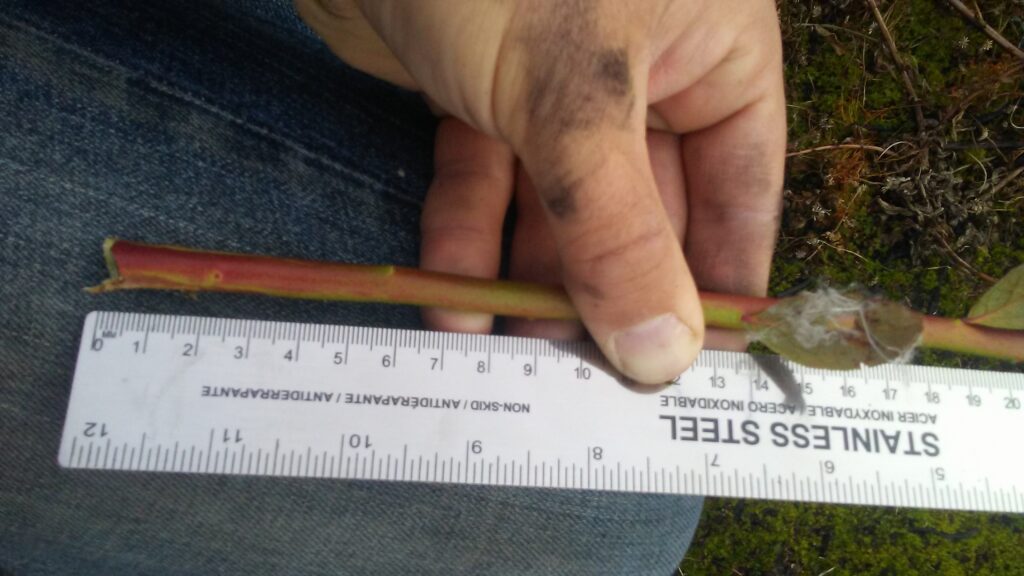
In the fifth picture I photographed the branch to be sampled while still attached to the original plant. According to my notes, the branch sampled had 42 nodes. If you can see the foot long ruler under the burnt blueberry bush, you’ll see that the branch is about three times longer than the ruler, so the branch had grown roughly a meter in one growing season. This may seem like a lot of growth, but many species of plants exhibit this response to having their canopy’s destroyed, especially ericacasious plants. In both the fifth, sixth, and seventh photos, we can see that the entire branch is composed of new, green tissues, and has virtually no lignified materials. Given the reports of fire in this area from last year (2018), the obvious evidence of recent fires in the immediate area (black suit, blackened peat, chard woody material, clearly visibly in all the photos) and the evidence of a single season’s worth of growth in the V. corymbosum plants, we can conclude with relative confidence that there was a bog fire in the summer of 2018 within the DND Lands, and, more importantly, in the areas where I will be observing plant fire responses.
Blog Post 5: Design Reflections
Although my data collection may be more straightforward then other studies that involve in depth measurements and larger study areas, I still found I had some difficulty solidifying my study areas. Due to the fact the pond I am studying is irregularity shaped it was difficult to create study areas that were the exact same area and consistent with one another (i.e. similar amount of grassed area, pond water depth, etc). I used air photos and online mapping tools to create a rectangle surrounding the pond and then divided the rectangle evenly in four. The quadrants were divided by direction which was one pro as that is consistent, NW, NE, SE, SW and will be utilized as a variable. I found it difficult to conduct accurate population density of the species by counting for the heavily populated species since it was difficulty to differentiate between individuals and keep track, to counteract this I decided to create a range rather than an exact number. This may be subjective and difficult to confirm accuracy, so I repeated this population count once a week for 8 weeks. There was little to no variation between each visit, especially with mature vegetation like trees. However, I also believe this information is bias to the current season being fall compared to obviously Winter, Spring and Summer. I am confident supplementary research will assist me in supporting my data and I look forward to research pond management and diversity further.
Blog Post 2: Sources of Scientific Information
Preliminary citations:
Davis, Neil, Rose Klinkenberg, and Richmond Nature Park Society (B.C.). Ecology Committee. A Biophysical Inventory and Evaluation of the Lulu Island Bog, Richmond, British Columbia. Richmond Nature Park Society, Richmond, B.C, 2008.
The PDF version of this study can also be found at: https://www.richmond.ca/__shared/assets/Lulu_Island_Bog_Report48892.pdf
Comments:
This particular publication goes into great detail about the flora of Lulu Island Bog, as well as fauna, endangered species, hydrology, effects of fire, soils, etc. It was authored by multiple authors, many are experts in their fields, including a number of professors. It was edited by Brian Klinkenberg, O.L.S., M.Sc., Ph.D., and is an Associate Professor of Geography at the University of British Columbia, and Rose Klinkenberg, who graduated from the Ecology and Field Biology program at the University of Toronto. Each section and chapter of the report deals with different aspects of bog ecology, and provide introductions, methodologies, results, discussion and conclusions, along with extensive in-text citations and bibliographies.
Of particular interest is the fact that this report states that the effects of fire in the Lulu Island Bog have not been well documented and require further study (pg. 248). It also makes mention of Scotch heather as an invasive species that responds with increased vigor after bog fires have occurred (pg. 96). So it may look as though looking at the intersection of bog fire effects, and the invasiveness of Scotch heather may be a relevant and timely aspect of this bog’s ecology to focus on, especially seen as how it just experienced fire last year, and has had one years worth of regeneration since.
Blog Post 5: Design Reflections
Reflecting upon my data collection, I did have some difficulties. A common, recurring issue that I encountered was human disturbance. To address this, I moved to a spot approximately 40 km from my home, located at the confluence of the Peace and Halfway Rivers. Eventually this area also became subject to significant recreational and industrial activity. This ultimately led me to cut my study short (e.g., 9 instead of 10 visits). Fortunately, I was able to collect a breadth of data. Looking at the data, it was somewhat surprising to see that certain species tended to be observed each visit but in relatively distinct strata within the overall study area (e.g., riparian area, floodplain, open water). If my study area had not become as subject to human activity, I would have changed my approach. I would have used the data that I gathered to pilot a study with a more focused approach both spatially (e.g., larger number of transects in each strata) and temporally (e.g., specific times of day over a shorter period) and probably focused on a single species. However, the repeated transect data that I collected will serve me well in small scale stratified study of occupancy. Further, I am still able to include hydrometric data as a variable in the analyses.
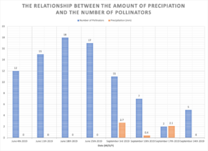
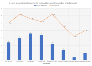
BLOG POST 8
So far I have made two graphs:
- The correlation between the number of pollinators and the temperature
- The relationship between the number of pollinators and the amount of precipitation (mm)
I think both of these graphs are perfect for showing my data that I have collected. I think my data is all normal, obviously it would be better had I recorded data for a longer period of time.