Based on my research so far the theoretical basis of my research is competition, niches, and succession. The areas I am researching have at one point been logged and so I am observing different levels of succession where the forest on the west side of the ridge has recovered from the logging event whereas the east side of the ridge has not recovered and is currently impeded by urbanization. The ferns are dealing with various levels of competition and different communities and so fill different niches in each treatment condition and have evolved to thrive in each niche to compete with the other plants. In addition, there is likely a difference in diversity between the three treatments since old-growth forests may have more diversity than areas that have had a more recent disturbance. This means that high diversity would be expected on the west side of the ridge as opposed to the east side where the logging has been more recent. Furthermore, the ferns may have evolved so that ferns in the forest have bigger leaves in order to collect more sun versus the ferns in the sunlight condition, which have smaller leaves as they can easily collect sufficient sun for photosynthesis.
Some keywords that summarize this project are as follows: ferns; Tracheophyta; vascular plants; competition; niche; community; succession; Pacific Northwest; ridge; Galbraith Mountain; sunlight; shade; logging; new growth forest; urbanization; diversity; disturbance. These words were chosen based on the research I have conducted so far for this study as well as descriptors of the subject and its locations.
Setting up my study site and collecting my first set of data points was a fairly lengthy process and though it has turned out to be an exciting adventure, it has also been fraught with uncertainty and a bit of the mundane. Let me summarize:
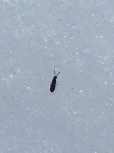
Organism of study: Snow fleas (springtails) in northern BC.
Hypothesis: Snow flea density on the surface of the snow is correlated with the presence or absence of cover/shade.
Prediction: Snow fleas will increase in density when given the opportunity to seek cover or shade in an otherwise open-to-the-sky habitat.
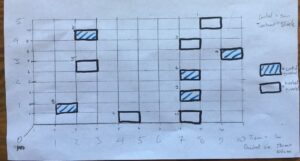
Figure 1. Simple Random study design. x and y coordinates generated at Random.org
Study design: I created a manipulated simple random experiment in which I took a 50m2 plot of open ground in my lower garden (5m x 10m) and divided it into 100 cells that could be randomly chosen to select 10 0.5m x 1.0m quadrats for observation of snow fleas. 5 of the 10 cells would be randomly selected for treatment (with a shade-producing tent placed over top), while the other 5 cells would be my control group (open to the sky).
For independence, I stipulated that no two cells could be adjacent to each other – I did not want the shaded quadrats to affect the unshaded quadrats.
I divided each 0.5m x 1.0m quadrat further into 50 cells in order to randomly select 5 10cm x 10cm samples from which I would count the snow fleas.
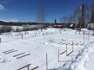
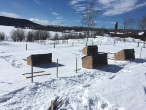
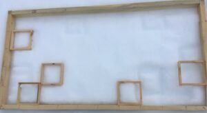
It took a few days of shop-work to create rectangle quadrats, tents and square sample units out of wood (this was the mundane part). When things were finally ready I set everything up outside and waited for the snow fleas to arrive. Figures 2 and 3 show how the site looked upon setup. Figure 4 is an example of one of the quadrats with 5 randomly spaced sample squares in it.
Figure 2. Quadrats in the snow.
Figure 3. Covered and uncovered quadrats.
Figure 4: One replicate with 5 sample units.
A few difficulties presented themselves:
After I set up my 5 treatment and 5 control replicates, all I needed was to count snow fleas, right? But they were no where to be found! Some winter days they seem to speckle the snow in truly astronomical numbers, and other days they are completely absent. Following my preparation for studying these mysterious organisms, they followed the latter trend – completely absent. The reasons for this, I believe, was that for the three days following my setup (March 9-11) we had morning temperatures of < -10C and daytime temperatures at around 0C. Apparently, they don’t want to rise to the top of the snow if it is too cold.
Cold but sunny days followed the setup of my wooden structures. The wooden quadrats and sample squares started to melt into the the snow, which I had carefully tried to not disturb in any way so as not to introduce confounding variables. The surface of the snow under the shaded coverings also seemed to be forming a different sort of crust than the surfaces left out in the open.
Anxious to get some data collected, on March 11 I went and collected my first round of data, randomly selecting new spots for the sample square placements and counted a total of ONE flea out of 50 sample sites! And it was in one of the sunny quadrats, not the shade like I had predicted! Was it now too late in the year to see snow fleas on top of the snow? Was I going to have to come up with yet another study idea?
The next morning (March 12) I noticed on my way to work that the temperature had barely dropped below the freezing point. Throughout the morning at my place of work, I noticed snow fleas in large numbers hopping all over the snow. I was informed by certain helpers that my study site back at home was alive with snow fleas as well, though interestingly they seemed to be avoiding the shaded sites and were sticking to the sunnier areas. Returning home, I was able to randomly select new sample points and start counting by 15:00, and at last had a data set that I was able to draw some conclusions from – even though the density numbers were not as high as I had envisioned or would have liked. I counted more snow fleas in the control quadrats than in the treatment quadrats.
Was the data I gathered surprising in any way? Yes, frankly. During my initial observations, it seemed like snow fleas were present in higher numbers in the forest and under shade compared with open areas. In my study site, they were present in higher numbers in the control quadrats that had no coverings, and were almost not present at all under the tents that I had erected. Nevertheless, the fact that there was a noticeable difference between treatment and control encourages me to believe this study design might have some statistical significance, and I would probably choose to continue pursuing this approach to data gathering.
That being said, I am also interested in adding another layer to the snow flea study (though this may or may not occur depending on time and scope for the purpose of this course): modifying the snow depth at each quadrat site and eliminating the shade factor, so that the explanatory variable now becomes continuous in nature – snow depth in cm. The response variable would remain the same – density of snow fleas. This interests me because during those times when snow fleas are most abundant, they usually seem to congregate in places of distinct disturbance such as boot-prints. Because they are soil organisms and rise to the snow surface from the soil it would make sense that they exist all throughout the snow column and densities are probably greatest in lower snow-depths.
My research project is examining the expansion of a stand of Trembling Aspen Populus tremuloides into a field at Campbell Valley Park in southwestern BC. According to some preliminary research I have done soil quality, sunlight availability (Romme et al., 2005), climate change, fire suppression, grazing and human interactions (Widenmaier & L Strong, 2010) are all potential factors for tree encroachment. The Aspen tree is one of the most common deciduous trees in North America and can reproduce asexually producing shoots that travel under the soil and produce cloned trees as large in area as a few acres(Mitton & Grant, 1980). Aspen are considered early succession species that take advantage of disturbed environments (Romme et al., 2005). Therefore, some keywords that would describe my research project would be early succession, tree encroachment, environmental gradient.
References:
Mitton, J. B., & Grant, M. C. (1980). Observations on the Ecology and Evolution of Quaking Aspen, Populus tremuloides, in the Colorado Front Range. American Journal of Botany, 67(2), 202–209. https://doi.org/10.2307/2442643
Romme, W. H., Turner, M. G., Tuskan, G. A., & Reed, R. A. (2005). Establishment, Persistence, and Growth of Aspen (Populus tremuloides) Seedlings in Yellowstone National Park. Ecology, 86(2), 404–418.
Widenmaier, K. J., & L Strong, W. (2010). Tree and forest encroachment into fescue grasslands on the Cypress Hills plateau, southeast Alberta, Canada. Forest Ecology and Management, 259(10), 1870–1879. https://doi.org/10.1016/j.foreco.2010.01.049
I am curious if the level of predator activity in an area affects the activity of a mole colony in the same area.
There are preceding works that provide a theoretical basis for my hypothesis. Some propose the use of models such as the Lotka-Volterra Model (Abrams, 2000) to show the relationship between predator and prey. This body of research creates an architecture around how to model predator and prey communities. The intent of my research is to identify if a relationship exists, and possibly what influences there may be on the communities in the WURA. Previous research paper’s such as this allow me with a basis on which to compare and contrast my own methods and results.
The focus of the research is on feral canines and feral felines acting as predators on eastern European moles in a semi urban setting. Some key words specific to my research project would be:
Mole
Canine
Predation
——————————————
References:
Abrams, Peter A. “The Evolution of Predator-Prey Interactions: Theory and Evidence.” Annual Review of Ecology and Systematics, vol. 31, 2000, pp. 79–105. JSTOR, www.jstor.org/stable/221726. Accessed 9 Mar. 2021.
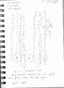
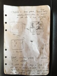
1.With switching locations, I’ve really had to brainstorm what I could study at this location. I’m quite interested in birds, but also vegetation. Upon observing this location, I found it interesting how the vegetation differs on one either side of the raise footpath considered the dyke, and the sides of the dyke. I’ve scanned some images below to highlight how the growth differs on each side.
2. That being said, I chose three parts of the dyke. The first is along the water with the left slant of the hill, the top of the dyke pathway, and the right slant of the hill along the farm border. From the water to the farm border is about 15 meters with 5 meters in between each spot.
3. Besides the different proximities to the water, I observed that the soil seems to be a little different. Particularly on the bramble side (left side) it was quite rocky with less concentration of dirt. Perhaps this is why grass does not prosper along that side? I also observed that around 14:10-14:48 in the afternoon, the sun does not shine on the left side. In fact, it was quite cool without the direct sunlight. When you compare plot A to plot B, the sun is direct, there seems to be a saturation of water in the soil (there was mud present). Plot C also seemed to have some saturation in the soil (a little soft), but not as much as plot B. Surprisingly, because plot A is along the water, although on the hill, there was not a lot of water present. Is this because the water directly runs off the hill and into the water?
I’d like to explore a hypothesis about the soil composition and how it supports the type of vegetation that grows on each plot as well as the amount of exposure of sun throughout the day on B and C.
My formal prediction: The soil composition along the dyke determines the variety of vegetation that successfully grows in each plot.
4. The response variable for this hypothesis would be the vegetation and it would be a continuous variable. The explanatory variables will be the soil composition and amount of saturation that contributes to the soil composition. This will be a categorial variable. I will use a one-way ANOVA experimental design for this study.
Field data was completed today. In total there are 30 replicates with 10 replicates of each condition. One of the issues that arose was that a few of the fronds sampled were eaten by insects or animals and so were shorter than expected. When processing data, these frond measurements will be excluded as they were shorter due to factors other than the amount of sunlight. Another problem I encountered was that it was exceedingly difficult to balance my lab notebook and measuring tape and so I acquired the help of a friend to record the measurements as I read them aloud. A third issue I encountered was trying to avoid stepping on other flora when walking towards and measuring the ferns. Otherwise, the data collection went relatively as indicated in my experimental design. The refinement made during the initial sampling was very helpful in making this process smooth.
One trend I noticed was that the eaten ferns tended to be in the shade treatment. While this does not change my hypothesis or alter it in any way, it is interesting and likely a result of the fact that the plants prefer the dense forest to sunlit urban backyards. Another factor I noticed is that the temperature is cooler in the woods than in the sunlight and I wondered if this was a factor in fern growth. Lastly, I noticed that in the shaded area there are a lot of plants and fungus including ferns, moss, trees, lichen, and other plants whereas in the semi-shaded area there was less variety of plant life as much of it lives on the edge of human activities. The sun area appeared to have a greater variety of grasses and other leafy green plants as opposed to the trees, moss, ferns, and lichen of the shaded forest. This does not change my hypothesis, but could potentially be a factor in accounting for the differences between the treatments.
The main difficulty with my sampling strategy was to do with the site locations. Before I began sampling, I went out to the field and used coordinates to document the areas where there were cedar trees (Thuja plicata) and where there were other trees but no cedar trees present. I then listed off all the coordinates and used a random number generator to select five sites of each type to sample. I planned to walk a number of paces (also generated by a random number generator) from the tree closest to where my GPS said I had reached my destination. This location would be slightly different from where I had taken the coordinates due to GPS inaccuracies caused by the forest canopy (Ordonez Galan et al., 2011). However, I did not take into account the level of imprecision, likely also caused by the tree cover. Instead of taking me to a precise destination as it would in an open area, the GPS only took me to about 20 metres away from the endpoint. To get around this, I began counting my paces from the tree closest to when the GPS had the lowest number of metres left to go.
The surprising part of the data was that the highest value of biomass collected was from a site with Cedar trees. Sample 3 with Cedar trees had a biomass of 580 g/m2. This value was inconsistent with the rest of the data collected from sites with cedar trees and is 28 g/m2 more than the highest value of the samples without cedar trees. I have gone back to this site and suspect that there are some confounding variables at play here. These variables include the amount of sunlight and the topography of the site.
I will be changing my data collection technique to take these confounding variables into account. To do this, I will ensure that the sites I document with coordinates are not in direct sunlight and have relatively constant terrain (no divots where water could pool). I will then continue to use a random number generator to select the sample sites. Another change that I will be making is to begin taking moisture samples alongside the moss samples. I will choose a day to go out and take soil samples from all the sites. Afterwards, I will weigh them, let them dry out and then weigh them again to find the moisture content.
Bibliography:
Ordonez Galan,C., Rodriguez-Perez, J.R., Martinez Torres, J., & Garcia Nieto, P.J., (2011). Analysis of the influence of forest environments on the accuracy of GPS measurements by using genetic algorithms. ScienceDirect, 54(7-8), 1829-1834
The initial data collection in Module 3 was done on a sunny afternoon. The sampling strategy chosen was to randomly choose ferns using random compass directions and random footsteps between 1 to 15. This was done in each of the areas chosen for study: full sun, partial sun, and shade. The data recorded was the number of fronds on the fern and the length of each frond. The fronds were measured with a flexible tape measure, which allowed for me to measure the frond from the very bottom of the stem to the tip of the leaf. The difficulty in my method of data collection was that I realized just how many fronds that ferns have. I ran out of space in my notebook, having planned for only 10 fronds. I immediately changed my technique when I realized that there were a lot of fronds so I sampled the first ten fronds starting with the frond on top closets to me and then going around in a clockwise direction until I reached that first frond again at which point I went to the second level of fronds and I continued in such a manner until I reached 10 fronds.
I was surprised that the shaded ferns seemed at a glance to have more numerous and longer fronds. I was similarly surprised that the partial sun fronds tended to have fern neighbors in contrast to the ferns in the sun condition.
As stated above, I had difficulty with the number of ferns and so adjusted my strategy. While I think that there is some bias in this method, I think that using the same method for measuring fronds will limit the bias. I think that this will improve my research as it means that there is a consistent process for measuring fronds. The randomization of selecting ferns appears to have worked, although I needed to be careful on the steep slope on the west side of the ridge and at times would have to repeat the random selection so I did not walk over a cliff. Otherwise, the method appears to be working well.
I have looked at a few ideas for study options up to this point. Most of my experience has been in forestry and vegetation, so a vegetation-based project was my natural first choice. The fact that it is winter here in northern BC and the ground is under a few feet of snow is one reason why looking at something other than plants is maybe a good idea. Here are some of my ideas up to this point:
I thought of looking at shrub abundance in relation to conifer crown closure, but this would require a truly landscape-level study.
I thought of looking at beaver presence-absence as a predictor for shrub and aspen-ramet abundance, but once again this would require being able to see evidence of beaver which would likely be under the snow.
I thought of looking at pine plantations and observing how young individuals grow bigger and taller in the presence of nitrogen-fixing shrubs such as alder than those individuals growing where alder isn’t so abundant.
What I’ve finally settled on is something truly fascinating and present in so many different environments in these parts – an organism I see all around my home as well as in the forests that I walk, ski, snowshoe, and work in. I will number the following points as per the blog instructions in order to keep everything easy to follow.
1) We (my family and the people around me) call them snow fleas but they are actually springtails, tiny arthropods that present themselves in different abundances all throughout the winter. In the order of Collembola, they come out on warm winter days and jump around on the snow and their bodies contain proteins that act like antifreeze to allow them to function in sub-zero temperatures (wikepedia). I would like to study their abundance and distribution in terms of density under different circumstances.
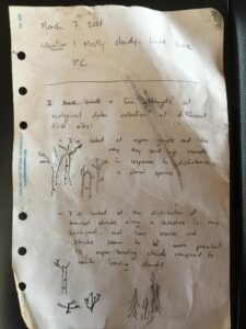
2) I will describe three environmental gradients in which I’ve observed them:
Open undisturbed snow in which (as of today March 7 2021) they were fairly uniformly and sparsely distributed.
Forested ground with crown closure where I saw they were quite a bit more dense, interspersed throughout bits of tree debris and forest matter
Disturbed snow, particularly relatively fresh disturbances like footprints from a few hours prior before new snow has fallen, in which they seem to congregate in large numbers, sometimes on one side of the footprint or the other which begs a couple questions. Are they seeking shade within the disturbance? Do they just happen to be in greater numbers because the disturbance has decreased the snow depth in that one place?
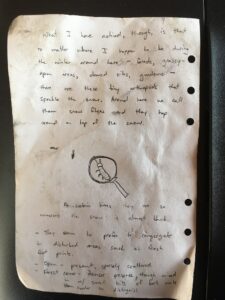
3.) As far as processes that may contribute to their relative abundance in different circumstances – open, closed or forested, and disturbed – there are likely several reasons:
As they are soil organisms, they are likely present in greater numbers over-top of ground that is richer or more nutrient-dense.
Snow-depth probably has a part to play – I would predict that as snow depth decreases, springtail density would increase.
Under cover of trees and with other bits of forest matter and debris scattered on the snow they would have more camouflage and be less visible to predators.
Direct or indirect sunlight may have an effect on their abundance.
One hypothesis I would like to explore – one that I think would lend itself to a study that would be possible to implement – is this:
Springtail density on the surface of the snow is determined by the presence of direct sunlight.
One formal prediction based on this hypothesis:
Though sunlight contributes to a warming environment conducive to springtail emergence, springtail density will be higher under cover or under a source of shade.
4.) The response variable in this case would be the density of springtails – this is a continuous variable. The explanatory variable would be presence or absence of direct sun (i.e. sun or shade) – this is a categorical variable. For this study, the experimental design would be a one-way ANOVA.
My field project study involves assessing the abundance of Broadleaf Stonecrop using percent cover in 1m2 quadrats along a few environmental gradients including elevation from sea level and micro habitat transition from shoreline to forest. My hypothesis is that Broadleaf Stonecrop abundance is determined by the moisture of the substrate which is indicated by a categorical level of drainability. Therefore I have predicted that the Stonecrop is most abundant in areas with high degree of drainability.
Thus far during my data collection I have noticed several ecological influences that may be affecting the abundance and distribution of my study subject. These would include exposure to sunlight, the underlying substrate, degree of slope within the growing area, substrate moisture content, as well as competition with other vegetation.
Since the Broadleaf Stonecrop is a succulent, they seem to thrive with very little substrate moisture hence my above prediction. They also thrive in areas where very few other vegetative species would be able to grow primarily steep, ocean exposed rocky outcrops along the shoreline. They also seem to require a high degree of sunlight and their abundance decreases dramatically in higher vegetated areas that would shade out the Stonecrop. Interestingly, it has been observed that the Stonecrop also only grows along the ocean facing cliffs in the study area, not the lagoon facing side.
Therefore both abiotic and biotic factors are having a direct and indirect influence on where the Stonecrop is most abundant. This study also touches upon competition for space and resources among various vegetation, adaptability in seemingly harsher environments, and higher tolerance for dryer conditions.
Three keywords that could be used to describe this study are climatic stressors, substrate moisture, and slope gradient.