Recent Posts

Blog Post 5: Design Reflections

User:  | Open Learning Faculty Member: 


Sample Date and Time: 2/7/21 10:40AM

For my initial sampling, I chose to use the systematic sampling method utilizing five 0.25 m2 quadrats spaced approximately two meters apart along a transect that ran in the heading of 110 degrees for approximately eleven meters. This transect was placed along my initially observed gradient of elevation from sea level. My initial sampling location was along the western rocky outcrop of the headland island. Within each quadrat, percent cover was recorded and indicated with one of five classes of percent cover ranges.

The most obvious difficulty for sampling the abundance of the stonecrop is and will be the accessibility to the sample points. As the stonecrop appears most abundant on the steeper rocky faces, some sample points may not be accessed safely and easily. When placing additional transects within each study area, this will have to be accounted for while trying to minimize sampling bias. Repeat transects within each study area will help minimize any bias from adjusting the transect locations.

My initial data collection generally agreed with my initial hypothesis that stonecrop abundance is negatively affected by increased substrate moisture as a higher abundance was measured at areas with well-draining, rocky substrate. However, it was noted that substrate alone may not be the best indicator as two samples that had rocky substrate had very little to no abundance of the stonecrop. It was also noted that the substrate type was generally consistent throughout the entire transect indicating that either a better predictor variable is needed or the transects should be longer (i.e run farther inland). The absence/presence of moss on the rocky substrate or degree of slope seem to be better predictors based on this initial sampling.

Going forward with full sampling I will continue to use transects and quadrats as these seem to be the most effective and efficient methods to capturing stonecrop abundance. Transect lengths will be increased which will necessitate additional quadrats. Each of the three study areas will have five transects with evenly spaced quadrats along each transect. An additional alteration will be to the percent cover classes used as my lowest class used (0-20%) may be too large a range to capture very small abundances.
Blog Post 6: Data Collection

User:  | Open Learning Faculty Member: 


Hypothesis:

The level of predator activity in an area does not affect the activity of a mole colony in the same area.”

Field Data Collection Activity:

Field data related to mole colonies and predators continues as I refine the process by which to conduct the collection. Originally I had intended on selecting a set mole colony inside of the Western Ukraine Research Area (WURA). However, the grid layout and detailed counts became unwieldy as I noted that the feral dogs would intrude during the longer time taken to gather data.

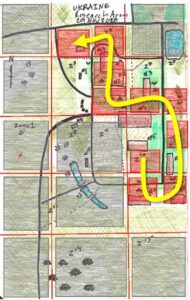
I altered my plan by researching point counts and how to conduct them in order to capture accurate information. Included in this process I laid out a routine path along which I will be conducting my data gathering. This consistency will improve the accuracy of my data.

Already I have tested this out and am using 10 replicates along a sampling route in the WURA. The intention is to do this for the next ten days in order to get the magnitude of data needed for a statistically relevant study. There will be ten repeats of the sampling process giving us 100 samples to work with.

Initial survey results show that there may be a correlation between predator activity and prey (mole) activity, but more data is required as ‘correlation does not imply causation’, especially in such a small sample count. It would be easy to jump to a biased conclusion before the data is completed.

Another alteration to my plan, is to identify the mole colonies as individual colonies rather than the zone identifications. Some colonies are in the same zones, so I will be labeling them as their own independent colony moving forward.

I am excited to continue the research project as I feel I now have an effective sampling method and there is a great deal of confidence that it will work well for what I need.

Fig. 1. Sampling path

Blog Post 5: Design Reflections

User:  | Open Learning Faculty Member: 


Previously I had been gathering raw data on mole hill activity and predator signs in a 1km x 1km area in western Ukraine. This area was divided into zones each with distinct boundaries and each with a mole colony. The northern half of the area has increased feral canine and stray cat activity.

The intent is to use the data to determine its effect on my null hypothesis, “The number of predators in a given area does not affect the activity of mole colonies in the same area.”

Initially I was using a haphazard sampling technique but had to refine it in order to capture moving pr

Example of Zone observations
Fig 1. Example of Original Zone observations

edators. The original sampling technique worked well to capture mole activity via the count of new mounds, but failed to be consistent in how predators were recorded.  The initial counts were also difficult to conduct because of the duration I was spending at each of the approx. 12 zones. This took most of the morning each day since I was gathering a large amount of spacial data. The time expenditure was significant. There was additional difficulty as I needed to gather data along a chronological gradient. Since the activity of the predators appeared to ebb and flow I also realized that this would need more than a single day of data gathering to do a comparison.

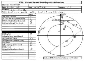
I wanted to capture statistically relevant data, so that I could determine if there was a correlation between these two data points. My solution was to pivot and use a point count with a 3 minute waiting period before moving on to the next location on the route.

This method would be more beneficial as the time frame would give me an opportunity to not only be consiste

New method of sampling
Fig 2. New point count method of sampling.

nt in the time of recordings, but also expedite my data collection.

After doing this I graphed some of my data and was surprised that there may (initially) be a correlation between canine predator activity and mole hill activity.

Continuing forward, I will collect data using the point count system. My hope is to do a week or two of data collection each morning to capture both the fluctuations in mole and predator activity. This alteration in data collection should improve consistent precision in my data gathering while reducing time spent.

I am looking forward to collating all of the data and seeing the results.

Blog Post 5: Design Reflections

User:  | Open Learning Faculty Member: 


Jan 23rd       Time: 2pm             Temp: -2 degrees

Weather: Windy 

Site: Kenna Cartwright Park

Originally, the sampling method selected was the belt transect and the trees that were being studied were both the ponderosa pine and douglas fir. The trees were counted in 50×10 m transects. Only the trees on the upward slope (going towards the top of the hill) were counted due to the scarce evergreen tree cover on the downward slopes. The belt transects were the sampling units and they were collected at 10 random distances in the 1000m from the entrance to the park. This sampling method was too broad and did not take into account other factors; data obtained would incomplete. 

The revised sampling method still involved 10 replicates over the 1000m distance from the entrance point. Only the Ponderosa pine trees were observed in this method. At the sampling points, trees in the 5m radius of the point were observed and the average diameter at breast height (DBH) was determined. Only the trees that are on the upward slope were considered. The distance from the entrance, the average DBH, the highest DBH and the elevation were recorded. 

The change in the approach enables analysis of the relationship between anthropogenic activity and the stability of the environment for tree growth while taking into account other factors in the environment. 

Instructor: Robyn Reudink

Post 9: Field Research Reflections

User:  | Open Learning Faculty Member: 


Overall I really enjoyed my field experiment. I learned a lot about aspen trees and gained a new respect for a tree that I honestly found annoying before this project. I now have a deeper understanding of the amazing ability of nature to not just survive but to find the best way to use the situation to thrive. My initial troubles with my project were limited to how I was measuring the green color. I was frustrated by my inability to accurately measure the chlorophyll layer but once I modified my approach I had no further problems. Completing this project has definitely made me more aware of the world around me and made me more curious about why other things may be the way they are. This project has caused me to look at things differently and to try and see the patterns and possible reasons for the events that take place in the environment around me. I have a much deeper appreciation for ecology and the knowledge that is gained through this area of study. This project has inspired me to want to investigate other aspects of my environment and keep learning and growing.

Post 8: Tables and Graphs

User:  | Open Learning Faculty Member: 


I do not feel that I had any trouble organizing my data. I would have liked to be able to more accurately measure the thickness of the green layer in the bark but lacked the needed equipment. I would have also liked to sample more locations but without a way to travel into the forest in the snow it was not possible. The data I was able to collect was fairly straightforward to organize as I was just measuring the presence or absence of the green color on the trunk of the tree. I was surprised by some of the data that I collected. I found that while most of the trees sampled had green only on the south side as I predicted, some had green all the way around the tree while others had none visible. I also found that elevation could be a factor in the amount of green as the trees sampled from higher elevations had a deeper color of green likely indicating a thicker layer of chlorophyll. This could be due to the harsher conditions and increased length of winter present at the higher elevation. Further exploration would be useful to determine if there was any impact due to the clonal nature of aspen trees. It could be that some trees did not have any noticeable green pigment because some of the surrounding trees with better access to sunlight were supplying other trees in the family group with energy. I would also like to further investigate if the age and circumference had any relation to the color. I did notice in my results that the smaller trees were a darker green as well as being green further up and down than the bigger trees. This could be due to their smaller root system and not having access to as much of the surrounding resources as the larger, more established trees.

Post 7: Theoretical Perspectives

User:  | Open Learning Faculty Member: 


My research project was to examine the presence of a green color on the trunk of aspen trees. My hypothesis was that the green color would be present only on the south side of the tree trunk in order to maximize sun exposure. The green indicates the presence of chlorophyll which trees use to perform photosynthesis. Photosynthesis is necessary for the trees to produce energy and is especially needed in the winter during the harsh conditions. The presence of the green color could be an indication that the trees are still able to photosynthesize in the winter without the presence of any leaves. This ability could give them a competitive advantage over other deciduous trees that do not have this ability. This ability would also likely improve the winter hardiness of the tree and give it a head start on leaf production in the spring which would allow the tree to make leaves ahead of others again giving it a competitive advantage and possibly blocking the access of other plants to the sun. This ability could also translate to increased reproductive fitness and overall increased survival rates. While I was collecting my data I also noticed that there was some variation noted in regards to tree circumference and the presence or absence of green color as well as related to the presence of surrounding competition and access to sunlight. I look forward to analyzing the data to see what I can learn from it. Three keywords I would use to describe my research project would be competitive advantage, winter survival, and resource sharing.

Post 6: Data Collection

User:  | Open Learning Faculty Member: 


I would have liked to be able to get further into the forest for at least some of my sample areas but the season and level of snow made that option unavailable. Sampling trees that do not have human interference in their immediate environment would help minimize the impact of some confounding variables. I chose the trees using the haphazard technique and sampled at least three replicates in each area. In total I sampled trees from five different and distinct locations in the local area. I did notice that the results seemed to be dependent on more than just the direction of the sun. It seems other factors could be influencing the location of the green color. It could be that there are more variables than I originally thought. I hope to find some other possible explanations after compiling all the observations.

Post 5: Design Reflections

User:  | Open Learning Faculty Member: 


When I initially planned this experiment I thought I would be able to determine different shades of green present on the trees. I had planned to match the tree trunks to a color wheel and see different shades of green. After making my first few attempts at data collection I quickly realized that this method would not work. Different viewing angles changed the lighting on the trunk and that alone changed the color. It was also difficult to determine different shades depending on what was around the tree or even in the background. I decided this method was too subjective and changed from my continuous approach to a categorical one to make observations just on the presence or absence of green on the tree trunks. Some of the data I collected did surprise me. I did not expect to see green all the way around the trunk on some trees. I also didn’t expect to see it completely absent on others. I plan to continue to collect data based on the presence or absence of color. I feel it is the best method I have without access to more expensive and accurate ways of measuring the green layer. Ideally I would be able to cut out small samples of bark and measure the thickness of the chlorophyll layer to get a truly accurate measurement as well as see if it was present in the areas where it wasn’t visible to the human eye.


Post 4: Sampling Strategies

User:  | Open Learning Faculty Member: 


I found the virtual forest tutorial quite interesting. The results were not at all what I expected they would be. The technique with the fastest estimated sampling time was the systematic but I was surprised to see how close all three techniques were. For the two most common species the sampling technique with the lowest percentage of error was the systematic and the highest percentage was the random technique. For the rarest species, the lowest percentage was the random technique and the highest was the systematic. When comparing the three strategy results I noticed that the systematic samples had not picked up any Striped Maple at all. It would seem that the systemic technique may not be the most accurate for the rarer species as it is possible to miss species populations completely. It also makes sense that the systematic system worked so well for the common species. My percentage of error for Sweet Birch was only 1.3%. The species that are common would likely be spread throughout the area being sampled. They would also be present in higher numbers making it more likely that the population will be represented accurately in the samples collected. The systematic technique is not as accurate for rarer species and the random technique was overall the most accurate although not by as much as I had thought prior to this exercise. I think having more sample locations would have increased the accuracy of all the results but especially the results from the less common species. It is too easy to miss the small populations when using small numbers of samples.