Recent Posts

Post 3: Ongoing Field Observations

User:  | Open Learning Faculty Member: 


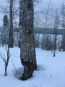
1) I plan to investigate the presence of green trunk pigmentation in aspen trees. I would like to determine if it is present on all aspen trees or if there are factors affecting the distribution.

2) My initial observation area only contained one small stand of aspen trees. Since aspen trees in close proximity to one another are often clones of each other, aspen trees from other areas would need to be observed in order to have independent replicates. I chose five different areas to observe aspen trees. The distance between the areas ensures the populations were independent of each other. Once I arrived at an area, the trees were chosen haphazardly mainly due to accessibility. I also had to choose areas that were accessible at this time of year by car as well as areas that had trees in snow shallow enough to be accessed on foot. Since accessibility was a concern, all the sample areas were located in close proximity to roadways or plowed parking lots.

In my first sample area I observed that the green color was present on the south east side of the trees but was not visible on the remainder of the trunk circumference. I observed three trees in this location and found them all to have the same green distribution pattern. The trees in the first area were in an open field on the edge of a cliff above a riparian area and had no competition for light or nutrients. Based on the observations from the first area, I wanted to see if different levels of competition/vegetation type, elevation, or direction had any impact on the presence of the green color.

The second area I observed was approximately 1.5 km from the first. The vegetation in this sample area was populated with both coniferous and deciduous trees. This type of vegetation provided much more competition for light and nutrients than was present in the first area. Five trees were observed at this location and all had green pigment present. The coloration was observed to be mainly on the south east sides of the trees and didn’t start until approximately three feet up the tree. Two of the trees were in denser areas of the forest and the green color was observed to be all the way around the trunks on these two trees. The bark on the larger, older trees was not green on the north side since this side is typically very rough and black so green pigment would not be visible.

The third area was the furthest away and the highest elevation. The trees in this area were again in a forested area with competition as well as being in a harsher environment due to the elevation. Winter in this area typically lasts longer and has much more snow than the other areas sampled. All the trees sampled in this area were green all the way around the trunk. One tree on the edge of a clearing had darker green coloring on the north side of the trunk. This tree was on the edge of a small clearing and had no immediate competition on the north side.

The fourth area was similar in climate to the third area but the trees in the fourth area were in the open with minimal competition. The trees with the smaller circumference in this area were found to be green all around and for most of the height that was observable with the south east side being a darker shade of green. The larger trees were a much lighter shade of green. One of the trees sampled in this area was next to a light that came on at dusk and off at dawn. This tree had very limited green visible.

The fifth area was on the edge of a marsh. The trees in this area were in the open with no tree competition and plenty of access to resources. They were located in town so may also have be impacted by artificial light. The green on these trees was noticeably darker on the south west side of the tree. The trees in this area did not have black scabby bark on the north side and they had branches growing almost uniformly on all sides. The trees in this area were observed to have green pigment present on their branches as well.

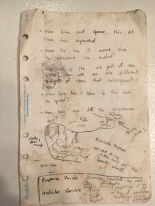
3) The patterns I observed could be caused by competition from surrounding vegetation, access to sunlight, exposure to artificial light, age of tree, or elevation.

My hypothesis is that green pigment will be present on the south side of all aspen trunks. I predict that the aspen trees will have green pigment on the south side of the trunk to maximize its access to sunlight.

4) One response variable is the presence of green coloring on the trunk of the aspen tree. An explanatory variable would be surrounding competition for sunlight. In this experiment the response variable would be categorical and the explanatory variable would be continuous.

Post 1: Observations

User:  | Open Learning Faculty Member: 


Initial Field Observations

Date: January 12, 2021           Time: 2:00pm – 2:30 pm                     Temperature: 0°C

Weather: overcast                   Location: yard around my house        Season: Winter

Side view of initial observation area

Aerial view of initial observation area

The yard is approximately 2.5 acres of flat grassland with a few trees along one edge and neighbors and a road on the others. The treed edge is the edge of a cliff leading down to a riparian area along a creek in the valley below. There is a beaver dam built in the creek below the house. Across the road is a mountain slope up to a plateau. The area is agricultural with most of the surrounding properties having various types of livestock.

The entire yard is covered in snow. No fresh snow for the past few days and snow on the ground has a hard crust. Minimal vegetation visible. Front yard has one large willow tree and a small lilac bush. The back yard has a large Blue Spruce, a small stand of Aspen on the cliff edge, and a small maple tree. Dormant Saskatoon bushes between the road and property edge. No dead grasses visible due to depth of snow. A few cones visible under the Blue Spruce in the back yard. No animals were observed during this observation session. No tracks, scat or evidence of any animals seen.

When examining the willow tree, many rows of fairly uniformly sized and spaced holes were discovered in the bark. Three small mushrooms were also observed to be growing on the willow but I was unable to tell if they were currently alive. An old bird’s nest was also seen in the branches of the willow. Bark damage to one of the aspen trees on the cliff edge was noted and photographed. The bark of the aspen trees was also noted to be green on some sides of some trees.

Holes in willow tree

Three questions that could be investigated further:

1) Holes in the willow tree: What made them? How can they make them so uniform? Why?

2) Green aspen bark: Why is it green? Why isn’t every tree green? Why only on some sides of the tree?

3) Mushrooms on the willow: Are they alive in the winter? If so, how can they stay alive in winter conditions?

Blog Post 2: Sources of Scientific Information

User:  | Open Learning Faculty Member: 


The source of ecological information I have chosen to evaluate is “A note on the observable bark coloration of quaking aspen (Populus tremuloides)” from the Western North American Naturalist.

Using the course information on how to evaluate sources of scientific information I would classify this article as academic, peer-reviewed research material.

This article is academic because both authors are associated with the University of Colorado. The article also contains in-text citations and a list of all cited literature. It is peer-reviewed because it specifically mentions anonymous editors in the acknowledgment section of the article. This article is research material because it contains methods and results sections.

Article link:

Rabinowitz, Oren and Tripp, Erin A. (2015) “A note on the observable bark coloration of quaking aspen (Populus tremuloides),” Western North American Naturalist: Vol. 75 : No. 3 , Article 12. Available at: https://scholarsarchive.byu.edu/wnan/vol75/iss3/12

Blog Post 2: Sources of Scientific Information

User:  | Open Learning Faculty Member: 


The source I chose is “Plants of Coastal British Columbia including Washington, Oregon and Alaska” which was compiled and edited by Jim Pojar and Andy MacKinnon. I would classify this source as academic, peer-reviewed review material.


It is an academic source because it was written by experts from universities such as the University of Victoria and Simon Fraser University, and the B.C. Forest Service. It includes in-text citations and a bibliography on pages 511 and 512. This source has been “technically reviewed by George Douglas and Chris Marchant” (p. 7), showing that it is peer-reviewed. Finally, this source does not include results from a study so it is review material.


Works cited:

MacKinnon, A., & Pojar, J. (1994). Plants of Coastal British Columbia including Washington, Oregon and Alaska. Lone Pine Publishing.

Blog Post 1: Observations

User:  | Open Learning Faculty Member: 


My study area is about 10 by 10 metres just off of Tannis Way in Nanaimo. The area has three main sections: 

  1. A meadow of exposed conglomerate rock covered by a thin layer of moss and a few small plants that can survive on so little sediment. It also has a footpath where regular human activity has caused vegetation to not grow. This section is on a slant and doesn’t retain water well so the water runs down into muddy pools.
  2. Muddy pools that retain lots of moisture and have collected sediment. These areas are mostly covered in a thick layer of sedge (possibly Carex stylosa but it’s hard to tell since it’s winter) and have few other forms of vegetation.
  3. The last section is under tree cover and has much more diverse vegetation. The trees include Arbutus trees (Arbutus menziesii) and short Douglas firs (Pseudotsuga menziesii).  Underneath the trees is a thick layer of moss, small shrubs like salal (Gaultheria shallon), and low growing plants. Dead trees had lichen and mushrooms growing on them. It is interesting to note that there are no Western Red cedars (Thuja plicata) and the salal is very sparse which is unusual for this area.

This is an Environmentally Protected Area designated by the City of Nanaimo. I visited my study area for the first time on January 21, 2021, at 1611 hours. It is currently winter and that day it was 5°C with a slight breeze and a clear sky.

Some possible questions for my research project: How do the differences in types of moss and thickness of moss affect animal diversity? How do the geographical differences affect plant diversity? What is causing the number of cedars and salal to be less than average?

Photo of the research area and some identified vegetation: https://photos.app.goo.gl/ASLsfzXSEjLjA3RE8

All vegetation was identified using:

MacKinnon, A., & Pojar, J. (1994). Plants of Coastal British Columbia including Washington, Oregon and Alaska. Lone Pine Publishing.

Post #4: Sampling Strategies

User:  | Open Learning Faculty Member: 


The Virtual Forests Tutorial revealed results that were surprising in varying degrees. I did the area based tutorial, and I think the most surprising aspect was that there wasn’t a single technique that produced the highest accuracy 100% of the time. While performing the tutorial, I thought that the random sampling method would produce the most accurate results because of the unbiased nature of the design: quadrats were scattered randomly throughout the entire study area as opposed to the single transect line of the systematic design. I assumed the haphazard design would produce the least accurate results (which it generally did), though I attempted to place the haphazard quadrats in spots that seemed “representative” or at least kind of random.

The systematic design had the fastest estimated time at 12 hours 4 minutes, which makes sense as it requires quadrats to be placed along a single line, or bearing. However it wasn’t faster by that much – all three sample designs were estimated to take between 12 and 13 hours.

As far as accuracy was concerned, the most common species encountered had the highest degree of accuracy in abundance estimates, and the accuracy of the estimates was relatively high in both systematic and random sampling placement strategies with random placement marginally the most accurate (except that it did not capture any data on the rarest species); the haphazard placements did not produce accurate abundance estimates for the common species. As a species abundance became scarcer, accuracy went down, except for the capturing of the rarest species (white pine) by the systematic placement of the quadrats, which (out of luck I presume) managed to pick up virtually all of the actual individuals in the sampling area.

Overall, it seemed like the number of samples was adequate to accurately quantify the most common species and would likely be sufficient in a relatively homogenous stand with uniform characteristics, but I would probably want more plots/quadrats if I was striving to capture rare species or a distribution pattern that was more clumped. If I could, I would attempt to use either random or systematic as my sampling placement strategy.

Blog Post 4: Sampling Strategies

User:  | Open Learning Faculty Member: 


After completing the virtual survey of the Snyder-Middleswarth Natural area, there were some interesting observations in regards to the time and accuracy for each sampling method in relation to the population density.

Survey Stats

Fig 1.0 – Survey Stats


OBSERVATIONS REGARDING DATA:

The technique which had the fastest estimated sampling time turned out to be the systemic transects at 12 hours and 35 minutes.

The percentage of error was lowest with the haphazard selection. This was surprising because it allows for inherent bias. When I conducted the virtual selection of survey quadrats, 5 locations were selected in the medial aspect of each topographical section, and spaced equally from west to east. This way a similar sample location was chosen along each topographical feature.
The fact that this was the lowest percentage of error is surprising as I was worried my bias would affect the outcome, but apparently because I applied a system it actually negated an increase in error.

The species abundance also affected accuracy. As the abundance decreased, we saw a decrease in accuracy. The accuracy could likely be improved with an increased sampling size. With any sampling, the lower sample size runs a higher percentage of error.

Overall the haphazard selection appeared to be more accurate than others, but likely due to the systematic bias I introduced by surveying plots equally distanced from one another in an almost grid shaped pattern.


Post #3 Ongoing Field Observations

User:  | Open Learning Faculty Member: 


I initially went out to my field site with the hopes of finding patterns in the way shrub species such as Amelanchier alnifolia and Salix were responding to browse pressure by moose. Looking at percent cover of biomass, horizontal growth patterns, or length of new shoots, I wasn’t able to imagine a study design that could answer specific questions, or maybe I just couldn’t formulate questions that lended themselves to good scientific study.

Thoughts on browse patterns

So I moved on to several places around my lake where Aspen stands have sent out suckers following beaver disturbance that ended some time ago, observing the gradient between the older stand and the younger individuals that have come up.

I also noticed other places where aspen were encroaching on fields or human-cleared sites, and some of these had distinctive successional gradients, too. And now to come up with a study design:

Aspen succession observations

1.) Identify the organism or biological attribute that you plan to study.

I plan to study Aspen trees in the process of succession.

2.) Use your field journal to document observations of your organism or biological attribute along an environmental gradient. Choose at least three locations along the gradient and observe and record any changes in the distribution, abundance, or character of your object of study.

One location is inside the parent clone of the aspen organism, where the individuals are mature with similar ages (presumably) and similar sizes (heights and diameters). Also noteworthy may be variables such as density, basal area, and incidence of health or pathological indicators such as conk.

Transition between aspen parent and offspring

A second location along the gradient is where there is an obvious shift in the clone’s attributes such as size, age, and density; i.e. where the aspen clone initially sent out suckers in response to the disturbance from years ago, and there is a higher abundance of individuals.

The third location along the gradient is the point at which there are no longer any suckers coming up, or where the suckers are obviously young or new clones, and maybe more abundant. In some places, shrub species are present in varying numbers/densities at this point on the gradient with varying levels of browse, and some of the aspen suckers are also being affected by browse pressure. Could the aspen be responding to browse pressure by continually putting out new suckers?

3.)Think about underlying processes that may cause any patterns that you have observed. Postulate one hypothesis and make one formal prediction based on that hypothesis. Your hypothesis may include the environmental gradient; however, if you come up with a hypothesis that you want to pursue within one part of the gradient or one site, that is acceptable as well.

Several processes are likely acting on the aspen trees to cause differences in the way they expand and fill the spaces they occupy following disturbances. Aspect, slope, and time are definite variables influencing the rate of aspen expansion I would think. I’m also curious about how the age and density of the parent stand at the time of clonal expansion influences how the younger clone individuals proliferate/spread. Many potential hypotheses to pursue…this project may incorporate the Hypothetico-Deductive Method approach.

I think I’ll start with age of the parent stand influencing how the younger clones develop. I hypothesize that the older the parent stand, the less its offspring will spread, or the less biomass will be produced by offspring. Framed another way, I hypothesize that the younger and “more vigourous” the parent stand is, the denser (or taller or further-travelled) the offspring will be.

4.) Based on your hypothesis and prediction, list one potential response variable and one potential explanatory variable and whether they would be categorical or continuous. Use the experimental design tutorial to help you with this.

Response variable: Density of the younger aspen. Or height to age ratio of younger aspen. This is continuous.

Predictor variable: Age of the parent stand. Though ascertaining the age of multiple trees would provide a continuous dataset, in this case (because aspen are clones) the parent stand’s age may be categorical, e.g. “veteran, mature, older immature” etc.

If I were to predict that offspring density or site index (a continuous variable) would be affected by the parent’s age as categorical, the statistical design would be ANOVA.

If I were to predict that offspring density or site index (a continuous variable) would be affected by the parent’s age in years (or density, basal area, site index – continuous variables), the design would be a regression analysis.

Blog Post 4: Sampling Strategies

User:  | Open Learning Faculty Member: 


For the virtual sampling tutorial, I chose to use area-based sampling for the Snyder-Middleswarth Natural Area. Results are shown in figure 1.

Figure 1: Virtual Sampling Results for 

As shown in the results table, all three sampling methods took over 12 hours to complete, with the random method being the longest at 13 hours and 13 minutes. The two most common species encountered were Eastern Hemlock and Sweet Birch, while the two least encountered (rare) species were Striped Maple and White Pine. Random sampling had the lowest percent error for the Eastern Hemlock, while systematic had the lowest for Sweet Birch. Systematic had a 100% percent error for the two rarest species, Striped Maple and White Pine. Haphazard had the lowest percent error for Striped Maple, while random had the lowest for White Pine, with haphazard only being slightly higher. Systemic generally improved greatly in percent error as species abundance increased. This was also generally true for random sampling as well. Haphazard did not show a consistent trend either way in terms of percent error with a change in species abundance as it greatly improved for the second rarest species but got much worse for the rarest species. For abundant species, I would say that systematic is likely to be the most accurate while haphazard would be the least accurate. For the rare species, systematic is likely to be the least accurate. With 24 sample points, haphazard was able to be quite accurate for Striped Maple but much less accurate for White Pine. This is likely a chance event and I would expect if this was repeated the percent error would be higher for Striped Maple. Likewise, systematic was not very accurate in sampling both rare species in which case increasing the number of sample points would likely improve the degree of accuracy.

Blog Post 9: Field Research Reflections

User:  | Open Learning Faculty Member: 


       This experiment was a combination of stress and pride as it was my first time designing and carrying out an entire research project! It was an interesting journey filled will multiple challenges and resulted in a project that I am very proud of.


        The major issue I ran into was weather changes. I was not prepared for how quickly the temperature declined this fall, and as a result, my variables may have been confounded. If I were to re-do this experiment, I would have began this as early as possible and completed my replicates while the temperatures were consistent. In addition to this, I would have adjusted how I approached my replicates. Instead of doing the replicates for each treatment on different days, I would have done them all in one day. This way, I would have had consistent temperature and weather, thus reducing confounding variables and improving the accuracy of my results. As a result of not doing both the the previously mentioned items, I had to change my second treatment from one flower to another. I chose to change the flower as my first choice was too withered to be considered viable for my experiment. Perhaps I will never know if this made a dramatic difference in my observations, but every consistent variable counts!


       This course and experiment has given me a much more engaging perspective on the scientific method and ecological science as a whole. The final project in conjunction with the textbook readings has evolved my appreciation for environmental science and I look forward to furthering my knowledge in this with future schooling!