Recent Posts

Post #8: Tables and Graphs

User:  | Open Learning Faculty Member: 


Everything surrounding the process of making the graph was straightforward and I knew already what kind of graph would best summarize my data, so all of this was smooth sailing. However, I was rather surprised when I saw the final result of my graph. I had an idea of what I thought the pattern should look like from the assignment earlier on in the course, but when I collected my data I thought there was no way my graph would even come close to replicating my prediction. I was ready to reject my hypothesis and was gearing up to take my study in the direction of exploring the other variables of why this hypothesis had no effect. However, upon seeing the final result of my graph I noticed that it was not anywhere to a close replicate, but the data did somewhat behave as I thought it would. Rather that moving in a smooth bell shape, it spikes up and down a little more than I thought, and I would love to find out what other variables were causing that reaction among my quadrats. And although it was a little more rigid, it does more or less follow the predicted pattern of starting moderately, rising and then descending to the lowest part of the graph. That realization was quite exciting for me! It made me really want to dive deeper into the other factors at play on this species in this ecosystem, as well as made me more fascinated by the cattails themselves.

All in all, I’m feeling very grateful for this class and this project for giving me a new curiosity in this field, and I’m very eager to finish the rest of the project and the class.

Post #7: Theoretical Perspectives

User:  | Open Learning Faculty Member: 


I am studying how the abundance of Typha latifolia affects the timing of their seed dispersal. First and foremost what I will need to consider in this study is the reproductive behaviour and processes of this species as well as how they behave with each other and with other species in their respective ecosystems. Whether their seeds are resilient and their reproduction is easily achieved will be crucial things to consider as well as whether they live harmoniously among other species both of their own kind and others. This will give me very valuable information in order to properly interpret my data. However, because ecosystems are complex and there are many variables involved, other factors begging to be considered are nutrient availability (because one would assume species with enough nutrients would reproduce more optimally than those malnourished) and environmental factors such as wind, temperature and light (because these are also things that could effect reproductive behaviour). What I aim to do in my research is find out when cattails best like to reproduce and find out if the amount of neighbors of their own species present has anything to do with the timing of their seed dispersal. Some keywords I would include for this study would be invasive species, seed dispersal, reproductive behaviour, and interspecies competition.

Blog Post Six: Data Collection

User:  | Open Learning Faculty Member: 


My data collection went fairly smoothly, similar to the collection we made of preliminary data. I did twenty replicates of 1M2 as planned to heighten the sample size. My sampling did however include some changes than what I proposed in my first small assignment because when I went to the pond to collect my data, I saw that one half of the pond had had all of the cattails completely levelled and removed. I was still able to space them approximately ten feet apart and maintained the sample size I wanted, however this means that one half of the lake was completely unsampled which is a shame because the two sides of the pond definitely differ in light as well as elevation from the pond and now I am not sure whether those are confounding variables that will influence the data.

Despite the fact that the collection process went smoothly, one thing I will note is that I can already see from the data that it did not progress as I predicted it would, and I am looking forward to analyzing it further and discussing why I think this was the case. One thing I also realized was that there are some large trees semi-nearby the pond that I did not factor into the abundance hypothesis, and I am not sure what effect if any they had on the data I collected.

Blog Post 3: Ongoing Field Observations

User:  | Open Learning Faculty Member: 


For my ongoing field observations, I visited Pipers Lagoon on Sunday, January 17th at 9:43 am.  The weather was overcast, 6 degrees in temperature, and no wind.


1. Identify the organism or biological attribute that you plan to study.

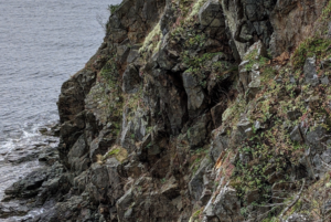
The organism I plan to study is the Broad-Leaved Stonecrop, sedum Spathurifolium.


Figure 1: Broad-Leaved Stonecrop
2. Use your field journal to document observations of your organism or biological attribute along an environmental gradient. Choose at least three locations along the gradient and observe and record any changes in the distribution, abundance, or character of your object of study.


During my first field observation, I had noted that the Broad-Leaved Stonecrop was generally only found along the ocean-facing rocky outcrops and not present on the lagoon facing ones. The plant is able to grow within various cracks and crevasses in the rocky outcrops. During this field observation, I decided to use the elevation from sea level as my gradient as well as exposure to the sun and the ocean. I also decided to focus on just the headland island portion of the park. 

I chose three different locations along the headland island, all with similar topography (open, exposed cliffs, primarily moss/lichen/stonecrop dominant). These were the northeast rocky outcrop, northwest rocky outcrop, and the south/southwest portion of the headland island. 

Figure 2: Observation Locations
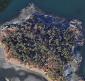
Along the rocky outcrop of the northeast side of the headland island, the stonecrop generally grew from mid to high elevation from sea level, with no growth at all below the high watermark. It was typically most abundant mid to high elevation, with less abundance along the plateau. As the amount of sun exposure throughout the day differed (i.e morning vs afternoon) it was noted that the abundance and distribution of the stonecrop increased (i.e more abundant and more area covered along the west side of the rocky outcrop than the east). Again, the growth was most pronounced at mid to high elevation and tapered off along the plateau. It was also noted that the stonecrop more exposed to the sun throughout the day had a more reddish color to its leaves than those that were in less sun-exposed areas.

The northwest rocky outcrop of the headland island had a similar growth regime (i.e mid to high elevation, tapering off at the plateau). It was noted that the stonecrop distribution spread beyond strictly the rocky outcrop on this portion of the headland island. A large abundance was observed along a steep slope farther inland than the rocky outcrop.

The Southwest portion of the headland island had virtually no presence of stonecrop, despite being a similarly rocky, sun-exposed area. However, there was certainly more soil and much less hard rock here than the more sea cliff type rocky outcrops in the other areas. This area also has no exposure to the open ocean while elevation gain from sea level was much more gradual and smaller than the much sharper increase in northeast and northwest portions of the headland island.


3. Think about underlying processes that may cause any patterns that you have observed. 


Some underlying processes that may cause the patterns observed include the moisture and drainage of the substrate that the stonecrop grows in, the type of substrate, and the amount of sunlight exposure.

Postulate one hypothesis and make one formal prediction based on that hypothesis. Your hypothesis may include the environmental gradient; however, if you come up with a hypothesis that you want to pursue within one part of the gradient or one site, that is acceptable as well.

Based on my observations of where the stonecrop was found to be thriving I hypothesize that stonecrop abundance is negatively impacted by increased substrate moisture. Therefore I predict that the stonecrop will be most abundant in areas with at least half-day sun exposure and bare, exposed rock.


4. Based on your hypothesis and prediction, list one potential response variable and one potential explanatory variable and whether they would be categorical or continuous. Use the experimental design tutorial to help you with this.


One potential response variable would be the abundance of stonecrop while one potential explanatory variable is substrate type. Substrate type would give an indication of the amount of moisture the stonecrop is exposed to as well as the drainability of water in the area. The response variable would be considered continuous (i.e abundance in terms of percent cover) while the predictor variable would be considered categorical (i.e type of substrate). This would classify the experimental design as being ANOVA.

Field Notes:

 

Blog Post 3: Ongoing Field Observations

User:  | Open Learning Faculty Member: 


For the course project I have been gathering data on the ecology and communities of a 1km x 1km area in western Ukraine.  The following information contains both my ongoing field observations and my considerations regarding a possible hypothesis.

Organism or Biological Attribute:
For the course project I have chosen to study the Eastern European Mole, and how it interacts with local predators such as dogs and cats.

Documentation:

I have been observing and documenting mole colonies, dog sightings, cat sightings, weather conditions, and mole hill activity over the last month in the observation areas. Specifically Zone 9, Zone 15, Zone 12, and zone 7.  Contrasting to this, there is a single Zone I have been documenting called ‘Control zone’ east of the observation area which has no Canine or Cat activity observed.

Example of Zone observations

Gradients Observed:

TOPOGRAPHY: In the control area, there is a gradient of topography with approximately a linear grade from the southern aspect dropping approximately 12 feet to the northern most aspect. Of note there is approximately an 8 foot gully near creek on western aspect of observation area.

VEGITATION: The general area which the moles are observed is the grassed areas which sit on a sandy aggregate soil.

PREDATORY CONCENTRATION: There appears to be a higher concentration of predators in north western aspect of observation areas, but less in south eastern area either due to topography,  territorial behavior, access to food, or a combination there of.

GROUND: Keeping in mind soil types change throughout the area. Again, the mole hills appear in sandy soil but the depth gradient of tunnels is not able to be directly observed despite the research on moles that indicates that these can go as deep as 6 feet. There is a carpet of decomposing leaves and rich soil under the oak trees (often thick with acorns) but little to none under pine trees.

TEMPORAL: Over time the count of active mole hills, spoor, coil conditions, and weather changes which may affect activity levels of all organisms in observation area.


Three locations inside the Observation area are:
——————————–
North west aspect of Zone 9 – Medium to low dog activity in area/transit point no sleeping
Northwestern Aspect of Zone 15 – Low dog activity in area as they adhere to eastern aspect for midday sleeping.
South eastern aspect of Zone 7 – High Dog activity due to transit+sleeping area
Central area of Zone 12 – Low mole hill count, high dog activity during midday.
Control area: Zero dog/cat activity – Zone A (east of map)

Area of Observation
Area of Observation

Processes and Patterns

Anecdotally the mole hills appear more populus and active in zone 9 and 15, as well as the control area to the east. This seems to be inverse to the dog activity in those areas. The temperature changes over time seem to affect the mole activity to some extent.

Hypothesis

The number of predatory dogs and cats in the area directly effects the activity of the colonies in the observation area.

Response variable(continuous): Mole hills along the gradient of dog activity.
Explanatory/Predictor variable (continuous): Number of dogs in the area (based on sightings and new signs)

Initially this appears that a study for this hypothesis would be of a regression design


Blog Post 4: Sampling Strategies

User:  | Open Learning Faculty Member: 


For the virtual tree sampling tutorial, I selected Mohn Mill. The three sampling strategies used were the Area haphazard method, the distance-haphazard method and the distance random/systematic method. The distance-haphazard method had the fastest sampling time.
The two most common species were Eastern Hemlock and Sweet Birch, and the two rarest species were the Stripped maple and White pine.
The haphazard area method had the lowest percentage error, while the haphazard distance error had the highest percentage error when used to measure the most common species.
For the rare species, the distance random/systematic method had the lowest percentage error, but no Stripped maple trees were located. The haphazard method had the highest percentage error.
The accuracy appeared to be decreasing with a decrease in species abundance for the haphazard methods. However, for the distance random/systematic method, the accuracy increased with decreasing species abundance.

Instructor: Robyn Reudink

Blog post 3: Ongoing Field Observations

User:  | Open Learning Faculty Member: 


Nov 22nd          Time: 1:30pm             Temp: 40C       Weather: Windy with overcast

Some of the dominant evergreen trees in Kenna Cartwright park are Douglas fir and Ponderosa pine. This project will be focused on the distribution of the evergreen trees with respect to the distance from the entrance point of the park.

These trees are easily identifiable, they have needle-shaped leaves, compared to the deciduous vegetation in the area that have lost their foliage.

Five different distances between 0 – 1000m were selected at which 50 x 5m belt transects were taken at the 5 different locations. These 5 distances were predetermined by an online number generator.

My prediction is that the density of the trees will increase the farther away from the entrance point. This may be due to the decreased human activity with an increase in this distance.

The response variable is the density of the trees and the explanatory variable is the distance from the entrance point to the park; this point is considered the zero point of measurement.

Since both of the variables are continuous, the regression experimental design will be utilized.

Blog post 3 images 

Instructor: Robyn Reudink

Blog Post 4

User:  | Open Learning Faculty Member: 


The results of the virtual tree sampling tutorial showed that the haphazard sampling method is the most efficient in terms of time spent, at a total of 12 hours and 30 minutes. This is in contrast to systematic sampling which took 12 hours 37 minutes and random sampling at 12 hours and 51 minutes.

Haphazard sampling is the most accurate method for common species. When measured with the haphazard method, the two most common species, Eastern Hemlock and Red Maple, had percentage errors of 3.34% and 29.7% respectively. In contrast, systematic sampling was the least accurate method for both species (18.3% for Eastern Hemlock and 41.3% for Red Maple).

Systematic sampling is the most accurate for some rare species but not others. For Striped Maple systematic sampling had a percentage error of 14.3% and for White Pine 185%. Random and haphazard sampling had a percentage error of 100% for White Pine.

For common species all sampling methods were relatively accurate. Accuracy declined for all methods as species rarity increased. The most rare species, White Pine, had the lowest accuracy for all sampling methods. For rare species, 24 sampling units may not be enough to get an accurate representation of their abundance. Therefore, although time consuming, increasing the sampling unit size may be necessary when studying rare species of trees and other plant life. Increasing sampling unit quantity would increase accuracy of abundance for all species, both rare and common.

Blog Post 2: Sources of Scientific Information

User:  | Open Learning Faculty Member: 


The source of scientific ecological information I have chosen to evaluate is “Linkage of Plant Trait Space to Successional Age and Species Richness in Boreal Forest Understorey Vegitation”, a journal article found in the Journal of Ecology Volume 103.


This article should be categorized as non peer-reviewed academic material for the following reasons:

The article is written by a number of experts, each with their own noted qualifications, working at prestigious schools. It has in-text citations throughout and contains a rich bibliography at the end. However, the article does not overtly identify a referee prior to publication as it does not contain any critique or evaluation.


Original Article Information:

Kumordzi, Bright B., et al. “Linkage of Plant Trait Space to Successional Age and Species Richness in Boreal Forest Understorey Vegetation.” Journal of Ecology, vol. 103, no. 6, 2015, pp. 1610–1620., www.jstor.org/stable/24542707. Accessed 13 Jan. 2021.

Blog Post 1: Observations

User:  | Open Learning Faculty Member: 


Saturday, Nov 7th     Time 2:30pm       Temp: -20C      Weather: Windy with cloud cover

I have selected Kenna Cartwright park as the site for the field project. This 800 Ha city park is located close to large shopping areas and transportation facilities in Kamloops. It is a mountainous and forested area with a variety of vegetation like the Ponderosa pine and Douglas fir, as well as some deciduous trees and shrubs. I walked 1500m along the path present in the park and observed the following:

  • Trees of similar maturity appear to grow close together; there is little observed heterogeneity in the maturity of the trees close to each other. I would want to study the relationship between the distancing of the clusters of trees and the probability of new tree growth.
  • The area above the path leading to the top of the hill has more evergreen trees while the bottom part of the hill has more deciduous shrubs. I would like to determine whether there is an observable difference in the composition of the soil between these two parts of the hill, which would affect the distribution of the trees.
  • The tree distribution varies with the distance from the entrance point. Considering that this park is close to high traffic and a developed area, I would want to study the relationship between the density of the trees and the distance from the entrance to the park, which is generally more accessible to disturbance factors

Images for Blog post 1

Instructor: Robyn Reudink