Recent Posts

Post 6: Ongoing Observations

User:  | Open Learning Faculty Member: 


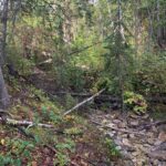
So far, my data collection has been going relatively well. The methods are easy to implement and I don’t have many physical obstacles that could hinder my study area. Zonation gradient does not seem to influence ant absence/presence as I found them in each ecotone, and elevation is not a factor to consider in my study because it is too minimal across the study site.

I am, however, finding that my data does not seem to fully confirm or support my hypothesis, as many factors affect patterns that I am to observe, and this will need to be addressed in the discussion of my research.

Some of these factors are:

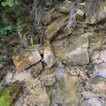
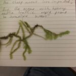
  • My predictor variables are not as straight forward as I anticipated; while vegetation cover could potentially affect ant presence, I found that it was most difficult to observe presence/absence in 100% vegetation cover of my quadrats. Additionally, disturbance was an issue and this was a significant flag when I noticed that pocket gophers created mounds of dirt of which were mostly present in the most vegetated zones, creating discontinuity. This type of disturbance favored my hypothesis only because the uplift of soil above the vegetation enables ant activity and exposure.
  • Precipitation is a factor that affects soil moisture (another predictor variable), however, the issue here isn’t the soil moisture as much as it is the daily precipitation, where they are not seen.
  • Another climate factor is temperature. As it is getting closer to “hibernation’ where ants start to slow down biological function, this phenological timing will affect my future findings. This might become another factor to consider in my data collection.
  • Lastly, The goal of my study is to identify if there is a correlation with ant habitat preference on an environmental gradient. Certainly, ant species behave differently, and hopefully this will not cause a fundamental flaw in my overall hypothesis.

Blog Post 9: Field Research Reflections

User:  | Open Learning Faculty Member: 


In reflecting on my experience designing and carrying out my first field experiment there were some aspects I really enjoyed, and others less so. I found a lot of satisfaction in the initial process of going out and closely observing nature. I liked that it embraced the principles of curiosity and the simple appreciation of being outdoors. I didn’t mind the process of picking a topic and designing my study, but I would’ve preferred doing it as part of a team. I believe my learning style is best served by having a team to bounce ideas off of, and particularly for my first field research project, I would’ve benefitted from working directly with someone else in the field. Admittedly, there were moments during the long hours of data collection when I was alone and morale was low.

That being said, I didn’t run into any real issues with the implementation of my project that required major changes, aside from adjusting quadrat sizes, equipment and minor alterations to my hypothesis/predictions, and am really appreciative of the experience. I feel that I have broadened my toolbelt so as to be better prepared for future endeavours in research and have definitely learned a lot regarding all the details that must be considered when developing a sampling strategy. Finally, throughout the data collection process I garnered a strong appreciation for the meticulousness, attention to detail, and patience that is endured in the development of ecological theory.

Blog Post 8: Tables and Graphs

User:  | Open Learning Faculty Member: 


I used a scatter plot to illustrate the relationship between soil moisture and percent slope from the data I collected. I ran into two primary challenges when creating my figure. The first issue I encountered was how to organize it in a way that maintained its clarity. I had 150 data points to plot on the figure, and after inputting them all I felt that the graph looked disorganized and busy, making it difficult to analyze. I tried to rectify this issue by including three extra plot points depicting the mean values across each of my three subareas, as well as trendlines, in an attempt to make patterns throughout the data more easily discernable. Inevitably, I don’t believe this was successful. The second issue I ran into was with my figure caption. I struggled with getting it properly formatted underneath my graph and additionally, I found it difficult to write it in such a way that explained my graph concisely. Word choice was difficult, redundancy as well as clarity were a challenge for me. I need to find a better way to more clearly describe which data was drawn from which subarea.

The data from my research were not totally consistent with my hypothesis. Soil moisture was, in fact, lowest where I thought it would be highest however, trees were largest at the bottom of the hill, as expected. Tree density was also highest at the bottom of the hill however, I predicted it would be highest at the midpoint. In terms of unexpected patterns, it appears that tree species distribution showed some degree of zonation across the slope.

Further research could explore this topic more in depth by measuring soil moisture within deeper layers of soil using more sophisticated tools, and look at changes in soil moisture as it relates to precipitation by collecting data at a variety of dates after a rainstorm to see how runoff might impact near-surface soil moisture across a slope.

Blog post 2: Sources of scientific information

User:  | Open Learning Faculty Member: 


Trophic ecology of alpine stream invertebrates: current status and future research needs.


This article on ecology is an academic peer reviewed review. The article is written as part of a doctoral dissertation in affiliation with a university (Fureder and Niedrist 2017); these authors can be considered as experts in the field.  It contains citations throughout and a bibliography at the end, this and the expertise of the authors makes this an academic resource. There is an acknowledgement to two anonymous referees making it a peer reviewed paper.  Finally, it would be considered a review as there is no methods or results section.


https://eds-b-ebscohost-com.ezproxy.tru.ca/eds/delivery?sid=45b0b78a-8552-49f4-9830-4bd75c899487%40pdc-v-sessmgr02&vid=10&ReturnUrl=https%3a%2f%2feds.b.ebscohost.com%2feds%2fdetail%2fdetail%3fvid%3d9%26sid%3d45b0b78a-8552-49f4-9830-4bd75c899487%2540pdc-v-sessmgr02%26bdata%3dJnNpdGU9ZWRzLWxpdmUmc2NvcGU9c2l0ZQ%253d%253d


Fureder L, and Niedrist G. 2017. Trophic ecology of alpine stream invertebrates: current status and future research needs. Freshwater Sci. 36(3): 466-478. Doi:10.1086/692831

Blog Post 4 – Sample Strategies

User:  | Open Learning Faculty Member: 


Below are the results of the 3 sampling strategies used in the virtual forest tutorial:


Virtual Forest Assignment Table Sampling Method
Species Systematic Random Haphazard
Eastern Hemlock

True: 469.9

Estimated: 408.0

Percentage Error: 13.2%

Estimated: 508.7

Percentage Error: 8.3%

Estimated: 388.0

Percentage Error: 17.4%

Sweet Birch

True: 117.5

Estimated: 92.0

Percentage error: 21.7%

Estimated: 130.4

Percentage Error: 11.0%

Estimated: 160.0

Percentage Error: 36.2%

Yellow Birch

True: 108.9

Estimated: 96.0

Percentage Error: 11.8%

Estimated: 78.3

Percentage Error: 28.1%

Estimated: 156.0

Percentage Error: 43.3%

Chestnut Oak

True: 87.5

Estimated: 124.0

Percentage Error: 41.7%

Estimated: 108.7

Percentage Error: 24.2%

Estimated: 100.0

Percentage Error: 14.3%

Red Maple

True: 118.9

Estimated: 140.0

Percentage error: 17.7%

Estimated: 126.1

Percentage Error: 6.1%

Estimated: 108.0

Percentage Error: 9.2%

Striped Maple

True: 17.5

Estimated: 36.0

Percentage error: 105.7%

Estimated: 13.0

Percentage Error: 25.7%

Estimated: 28.0

Percentage Error: 60%

White Pine

True: 8.4

Estimated: 0.0

Percentage error: 100%

Estimated: 0.0

Percentage Error: 100%

Estimated: 8.0

Percentage Error: 4.8%


  1. Based on the information provided, the fastest estimated sampling time was the random sampling method estimated at 12 hours and 19 minutes.
  2. The 2 most common species are the Eastern Hemlock and Sweet Birch. As you can see from the data presented above, the random sampling method yielded the lowest percentage error. For the 2 rarest species – Striped maple and White pine –  the random sampling method yielded the lowest percentage error for only 1 of them (Striped maple), whereas the White pine’s lowest percentage error was in the hap hazardous sampling method. The accuracy did seem to change with species abundance generally speaking.
  3. After taking the mean percentage error of each sampling strategy these were my results – Systematic (44.5%), Random (29.1%) and Hap Hazardous (26.5%). This would be indicative that the Hap Hazardous Sampling Strategy is the most accurate out of all 3 strategies.

Blog Post 3- Ongoing Field Observations

User:  | Open Learning Faculty Member: 


Designation: City Park, Community Garden
Time: 1647 hours
Date: 08-09-2020
Weather: Sunny, clear sky, hot and dry, minimal breeze 25 degrees celsius, hazy (Forest Fires in Effect In Washington DC)
Seasonality: Summer, approaching fall
Study Area: Community Garden at 1645 East 8th Avenue Vancouver BC. Latitude: 49.2635 Longitude: -123.0711. Study area is generally small, approximately 2 houses worth of lans (~1500 sq. feet)

The organism I plan to study is the Western Honeybee (Apis mellifera)
As briefly outlined in my field journal, I have chosen 3 locations along my environmental gradient (between the bee hive and street located about 25 paces South from the hive. For the sake of ease I have labelled the areas by the plant that I am observing the honeybees on there:

Location 1: Elderberry Flower Shrub (7 paces East of hive)
-Character: Bees seem to be busier, more movement observed in the bees between each small flower on the plant.
-Distribution: Bees are pollinating moderately closely together, seem to pollinate the flower bunches that are in direct sunlight. Not every flower bunch contains bees, out of 1 shrub approximately 3-6 flower bunches contained pollinating bees.
-Abundance: 5-7 bees pollinating on one flower bunch at any given time

Location 2: Small white flowers (11 paces South of Bee hive, towards street)
-Character: Bees are still pollinating here, don’t seem to move as quickly (perhaps this is just because I do not see as many bees in this location, giving the illusion that they are moving slower)
-Distribution: Bees are pollinating further apart than location 1, can count 3-4 flowers in between flowers that contain a bee pollinating it. the entire plant is in direct sunlight, no shaded areas to observe the difference of bee activity.
-Abundance: 3-7 bees on entire plant at any given moment

Location 3: Orange Flowers (21 paces south of bee hive, closest location to the street out of locations observed)
-Character: Bees still pollinating here, seem to be more “picky”, going from flower to flower until they choose one to pollinate. Seem to be moving as quick as they do in location 2
-Distribution: Bees pollinating far away from each other. The whole plant contains approximately 10-15 flowers and only 1-3 bees will be on the entire plant
-Abundance: 1-3 bees on entire plant at any given moment

3. After thinking about possible underlying processes that may cause the patterns observed I have come up with a hypothesis and prediction:

Hypothesis: Roads influence Honeybee pollination patterns

Prediction: I predict that Western Honeybees pollinate plants that are located furthest away from the street.

4. Based on my hypothesis and prediction, I have written one potential response variable and one potential explanatory variable:
-Response variable: Western Honeybee Activity. This would be a continuous variable as I can use numerical units to count the numbers of honeybees over a period of time that visit the site.
-Predictor/Explanatory variable: Distance from the street (East 8th Avenue, Vancouver BC). This would be a categorical variable.

Because my predictor variable is categorical and my response variable is continuous, this would be indicative of an ANOVA design. I hope to use a one-way layout design to compare the pollination activity of my 3 treatments.


Blog Post 7 Theoretical Perspectives

User:  | Open Learning Faculty Member: 


My research is primarily concerned with the presence or absence of conks growing on trees. This relates to tree health, possibly opportunistic pathogens, and succession of a second-growth forest.

An idea that underpins my research is conk prevalence in one area of Mundy Forest. Is it a natural environmental condition, is it there because of tree disease and is the tree decaying before the presence of conks or because of it? It also touches on disturbance regimes and the successional stages of the forest (micro-disturbance from the death of trees allowing more lower canopy growth with additional light availability). The typical forest structure of the Pacific North West includes an iconic species, Western redcedar, in which climate change is strongly affecting the typical forest diversity. Changes in precipitation, temperature and drought patterns are affecting the distribution and health of Western redcedar. This may be an idea underpinning my research of tree health or decline and may have nothing to do with conks.


Tree health, opportunistic pathogens, climate change, bracket fungi

Blog Post 4: Sampling Strategies

User:  | Open Learning Faculty Member: 


Virtual Forest Tutorial: Snyder- Middleswarth Natural Area.


Results of Sampling Technique Tutorial
Sampling Technique Systematic Random Haphazard
Common Species Actual Density (T) Estimated Density (E) Percentage Error % Estimated Density (E) Percentage Error % Estimated Density (E) Percentage Error %
Eastern Hemlock 469.9 460 2 304.2 35 375 20
Sweet Birch 117.5 124 6 100 15 137.5 17
Yellow Birch 108.9 68 38 129.2 19 95.8 12
Chestnut Oak 87.5 100 14 108.3 24 75 14
Red Maple 118.9 124 4 179.2 51 91.7 23
Rare Species
Striped Maple 17.5 16 9 0 100 20.8 19
White Pine 8.4 0 100 20.8 148 8.3 1


Time Spent Sampling:

Of the three sampling strategies, systematic, random, and haphazard, they were all very similar in the amount of time spent sampling, with haphazard being slower than the other two by 2 minutes.

Accuracy of each Method of Sampling:

The most accurate sampling method for the more common tree species was the systematic sampling method.  The most accurate sampling method for the rare species, Striped Maple and White Pine was the haphazard method. The accuracy for the systematic and random method declined for the rare species compared to common, due to the fact that they missed one rare species all together each. Whereas the haphazard method stayed about the same for both common and rare species. Perhaps with more sample points and another location for systematic would have been more accurate.

Observations 1

User:  | Open Learning Faculty Member: 


07/09/2020

08:47

8 °C overcast

-transition season with summer ending and moving into fall, rainfall in the past 24hours


The site is located on Steamboat Mountain and is designated as rangeland, specifically the Bryanton Creek and Tea Kettle ranges.  It is a mountain slope with primarily conifer forests. I chose three small perennial streams that flow through the area (Figure 1). Each of the sites shows recent use by cattle (Bos Taurus) with tracks and manure.  The slope to access the creeks at the point of observation is varied for each location; site 1 location 4 is forested and has little slope (Figure 2), site 2 location 2 is steep, rocky and has small areas of pooling (Figure 3), site 3 location 3 is gently slopped with steeper sides (Figure 4). The streams are rocky and varying sizes of pooling with gravel to muddy linings.  All three sites have similar vegetation with large spruce (Picea ?), birch (Betula papyrifera),and Douglas fir (Pseudotsuga menziesii var. glauca) forming the primary canopy.  There is an abundance of red-oiser dogwood (Cornus stolonifera C. sericea), common horsetail (Equisetum arvense), and bunch berry (Cornus canadensis) as well as mosses and lichens at all three sites.

Figure 1 Creek locations created on iMapBC

Figure 2 Creek site 1

Figure 3 Creek site 2

Figure 4 Creek site 3

Field notes

Questions that I had after observing these sites includes:


Is the health of the streams impacted by the cattle?

Is there concern with E. coli in the streams with the cattle defecating in the streams?

Does the access to the stream, as far as steepness, have an impact on how used the stream is by larger animals such as cattle and ungulates?

Blog post #5: Design Reflections

User:  | Open Learning Faculty Member: 


My initial sampling day went as planned insofar as I was able to collect data using the method of walking a transect and placing my quadrat after a random number of paces. I was even able to find my target species in some of the quadrats and record useful data. My sampling plan was flawed, however, as it assumed a higher density of dog strangling vine. I ended up covering the whole length of my study area before I was able to obtain 5 quadrats containing the target species. The issue is that, while abundant, the vine grows in a small number of patches. My initial design attempted to avoid sampling more than once from each patch by having a minimum number of paces, but this turned out to be a problem as there are only 4 patches in the particular treatment area I was sampling. Further investigation revealed the same issue in the other treatment areas. My study area doesn’t have enough Dog Strangling vine patches to be sampled in this way.

The response variable data collected was generally as expected. The number of seed pods on the plants reflected the different treatment areas as predicted in my hypothesis. The soil moisture or predictor variable measurements were not as expected. All of the soil was measured to be dry, regardless of the treatment area. During the sampling it became apparent that this was another flaw in the study design. To demonstrate that the slope or manicured areas had less water than the area along the creek (which seems to be the case based on the compaction and visual dryness of the soil), I would need data throughout the growing season that showed the plants consistently had less water. A simple snapshot would not demonstrate this effectively.

I am going to modify my sampling approach in two ways.

First, since my sample unit is the individual plant, I am going to sample the various patches in greater depth instead of using random paces and quadrats along a transect. This will provide several replicate areas within each treatment and allow for a larger number of individuals to be counted. A quadrat will be used within each patch to collect 3 or 4 separate samples, several meters apart from each other. A random number generator will be used to determine random locations within each patch for sampling.

Second, since I can’t demonstrate that water availability is different across time between the different treatment areas. I will have to rethink my hypothesis. The data supports the observation that there is a gradient in the number of seeds between the different treatment areas so the predictor variable will be modified to be the different treatment areas themselves within the study area.

These two modifications will allow for significantly more individuals to be sampled within the study area while maintaining random selection, and allow for a hypothesis that is verifiable or refutable.