My research project was a wild ride. Originally, I had planned to sample bryophytes on Mount Tolmie, which is a park that has an altitudinal gradient. In March when the pandemic hit, I left Victoria – where I was living and attending school – and I did not want to start my entire project from scratch. Earlier in my university career at UVic, I had learned about a website called iNaturalist and I wondered if I could use this website to help me collect data from my original space without having to be there. I ended up using citizen scientist data from iNaturalist in conjunction with some data that I had collected back in February of 2020. Because of this change, I had to make a lot of adjustments in my design and expectations for this project. Using iNaturalist was surprisingly easy, and I was able to get approximately 50 data points for use in my study. Since engaging in the practice of ecology I definitely have a greater appreciation for this field of biology, I have focused on cells and biochemistry for much of my education and never thought much about ecology, but this project opened a big door in my mind!
I had some issues with organizing my data, since it came from a crowd-sourced database. First, I had to decide which genera to include in the data set, and I decided on the three most commonly sighted. Then, I had to select the data that I was concerned with, being the coordinates of each sighting. From there, I used the coordinates to identify the elevation that each sighting was recorded at. Then, I used the number of sightings and elevation to form my graph, with elevation on the x-axis. The results were pretty much as expected, and similar but less evident trends to the graph I created with my predictions earlier on. Due to the small sample size that was available from the iNaturalist database, I would like to collect much more data and examine how the trends on the graph change. I would expect that they would be similar to what is present now but would be much more defined.
Bryophytes are an important component of nutrient cycling in ecosystems and therefore have an impact on soil composition and neighbouring vegetation. Because of this involvement, they have a significant impact on the biogeochemistry of the region (Cornelissen et al., 2007). Understanding biogeochemistry is important for creating a complete picture of the natural environment, and understanding when or why things grow in the habitat. Changes in bryophyte species richness may be indicative of underlying changes in biogeochemistry that are also associated with the change in elevation. Also, there may be a biogeochemical reason why some species are able to live at higher elevations, lower elevations, or all elevations.
Three keywords that I would use to describe my research project are bryophytes, elevation gradient, and biogeochemistry.
Cornelissen, J.H.C., S.I. Lang, N.A. Soudzilozskaia and H.J. During. 2007. Comparative Cryptogram Ecology:A review of Bryophyte and lichen traits that drive biogeochemistry. Annals of Botany. 99(5):987-1001.
Preamble: After reassessing my planned sampling methods and study site, I began collecting my formal data on August 5th, 2020. In this blog post, I have included information regarding some changes to my project. I have opted to include these updates in this post, rather that the original blog posts to avoid the need for the reader to navigate to my other blog posts to understand the context in which this data was collected.
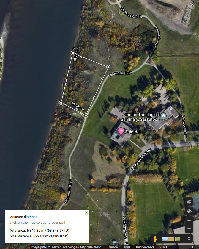
Study site updates: Due to the difficulty in navigating some of the steep slopes within my initial study area, and avoiding some areas that may confound the project, I have redefined my study site. The original study site was an area of approximately 38 576 m2 in size and encompassed a ravine. I desired to study the forb species abundance and distribution along the riparian-upland gradient on the eastern bank of the South Saskatchewan River. However, the ravine threatened to confound my project (having a separate species profile and elevation gradient), and some of the cliffs within the original study area were going to be too difficult to navigate. Therefore, the study area was reduced to 6 349 m2 and is depicted in Figure 1.
Hypothesis updates: My original hypothesis involved investigating forb species abundance and distribution as they relate to the distance from the river. However, I have now opted to shift my focus towards elevation (rather than distance). Furthermore, in an attempt to address the processes behind forb abundance and distribution, I have decided to estimate soil moisture along the gradient.
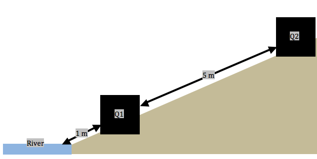
Sampling method updates: Following some advice and reflection on my proposed sampling methods, I have decided to adopt a systematic sampling approach (along transects) within the study area. Each transect will run perpendicular to the shore of the river and contain 11, 1 m2 quadrats that are spaced 5 meters apart (Figure 2). Ten randomly generated locations at the shore of the river were chosen and the first quadrat in each transect is to be laid at 1 meter from the river’s shore. Along these transects: I have been collecting forb species abundance, noting the proximity to river, estimating soil moisture (by hand texturing), and noting whether there is a tree/shrub canopy hanging over the quadrats.
Data Collection: Three replicates (transects) were sampled on August 5, 2020 between 9:30 AM and 6:30 PM. As stated above, each transect consisted of 11 sub-samples (quadrats).
Transects proved difficult to implement because the slope was extremely steep in some locations. Working from the river, I would lay a quadrat, collect data, then measure 5 meters to the next quadrat location. Some locations arose where I would not be able to move in a straight line (often up a cliff); therefore, I would have to mark the location of the previous quadrat, navigate to the new location via an alternate route, and measure backwards to maintain a consistent distance between quadrats. In addition, the upper area of the riparian zone is dominated by dense stands of Caraganasp. and Amelanchier alnifolia (Saskatoon berry) shrubs. This region was particularly time consuming to navigate; however, it was still feasible. The locations with a dense shrub canopy exhibited a notable absence of forbs. Therefore, at the sixth quadrat in transect one, I decided to begin noting when a canopy of shrubs or trees hangs over each quadrat. In order to maintain consistency, I navigated back to the previous five quadrats to collect this data before continuing to the seventh quadrat in the first transect. Overall, the largest problem in implementing my sampling technique was time. Not being able to complete all ten of my replicates in one day will mean that I may not have consistency with soil moisture between sampling days. This can be mitigated by ensuring that my sampling is, in the very least, completed within a timely manner (over the next few days). In addition, I will be navigating to some of my previous points on subsequent sampling days to verify that the moisture content of the soil has not changed. If it has, I will need disregard my previous soil moisture data and plan for an individual day of soil sampling to control for moisture variances.
Despite having only sampled from three transects, I am noticing ancillary patterns related to my hypothesis. The transects closest to the river are all saturated with water and this saturation level quickly declines as you move up in elevation. Consequently, many forb species exhibit preferences for different elevations. For example, Astragalus pectinatus (narrow-leafed milk-vetch), Cirsium arvense (Canada thistle), and Liatris punctata (dotted blazing star) display an extreme preference for dry (0-25% saturation), upland locations. In addition, Hedysarium alpinium (alpine hedysarium) and Astragalus americanus (American milk-vetch) are strongly associated with heavily saturated (75-100% saturation), low elevations. However, some forb species like Solidago canadensis (Canada goldenrod) do not appear to display a preference for any elevation or moisture content.
Figure 1: The figure above is an image taken from Google Maps depicting the redefined study area.
Figure 2: The figure above is a diagram depicting the location of the first two (Q1 and Q2) quadrats in a transect. Q1 is positioned 1 m from the river and every subsequent quadrat is placed 5 meters away from the previous quadrat, along a perpendicular line extending from the edge of the river.
REFERENCE LIST:
Google Maps [Internet]. c2020. Canada: Google Maps; [accessed 2020 July 29]. https://www.google.ca/maps/@52.1378074,-106.6412387,549m/data=!3m1!1e3
In module 3, I collected data for my experiment to understand whether the presence of other plant species (carrots, pumpkins, onions, and peas) have an influence on the growth and abundance of bean plants near (in 30cm distance) them. For the small Assignment #1, I chose one garden plot, to collect my data.
I selected the systematic sampling strategy to record data because it would help me to avoid the experimenter bias while choosing the samples. This also seems like the best approach because it would prevent collecting samples that are clustered in the same area, but instead use the samples that are spread out around the garden bed. The first individual bean plant sample was randomly selected, and then the next samples were systematically selected. From the fifth plant north, then the fifth bean plant East. However, the difficulty with this method was: the garden plot was not large enough for the samples to be spread out perfectly in fives. This is therefore why I plan to use the same approach, systematic sampling technique, but I will record every third plant instead of the fifth. Individual samples will still be spread out, and I will have the opportunity to record even more samples. Also, instead of collecting just the presence of other plants, I will also record what those plants are to be more detailed. This will increase accuracy, and provide more data for the analysis.
The collected data was somewhat surprising because the results were different from my predictions. I predicted that the closer the bean plant would be from these other plants, the more leaves and flowers it would have, which was not reflected in my data. I started to suspect that my hypothesis might be falsified, but I will not know until I collect more data. This opened my mind to think about possible confounding variables.
Some of the confounding variables that could play a role in the abundance of these bean plants could be the type of soil, moisture levels, type of bean plants and planting dates especially between the different garden beds. I will do more observation, and to avoid these possible confounding variables. An approach I plan to take to avoid these confounding variables is to firstly compare the bean plants within the same garden beds, before I could compare the beans in different garden plots who might not share some of these factors.
Finally, more careful observation will increase certainty of more extensive data to be collected on the next trip. In addition, a more detailed recording of data will provide more meaningful data that will lead to a more accurate conclusion.
On August 3rd and 4th i collected the data from the remaining three of my four 10 x 10m sample plots, located along the shoreline of Nita Lake. Each sample plot was a replicate. Starting with Plot 1, i put into practice my now slightly more refined technique for determining elevation, with the series of 1 meter vertical poles and string running horizontally until it meets the slope of the shoreline. In the sub-1 meter elevation zone, Alnus rubra grew densely and i had trouble counting the individuals without accidentally backtracking and double counting. However, i started flagging each tree as i counted them and walking up and back parallel with the shoreline boundary of the plot, recording the trees as i gradually made my way up the slope until i hit the back line of the plot. This made it much easier to ensure that i had an accurate tree count, without double counting or missing any individuals.
I have noticed that the substrate types in the sub 1 meter elevation zone are uniform across the four plots, which i believe could be a result of frequent flooding and erosion, creating deep, soft and moist soil substrates in the low lying areas. This could potentially compromise the testing of my hypothesis, as Alnus rubra dominance in low lying areas may be influenced by substrate type rather than correlating only with frequency of flood disturbance. However, for this reason i recorded all changes in substrate types throughout the different elevations, so by analyzing the species composition in different substrate types throughout sample plots i should be distinguish and nullify the influence of substrate type in the flood prone zones.
I decided to study vegetation diversity with increasing distance from the creek in my home town. My hypothesis was that proximity from the creek would effect the variety of plant life growing in the area. I predicted that, as distance from the creek increased, the variety of vegetation would also increase. I predicted the heardier plants like the Cows Parsnip and grass would survive closer to the creek because they are typically able to survive in a variety conditions. They can grow in shade or direct sunlight and in damp areas as well as drier areas. Other species, such as the wild rose, needs to have a bit of shade as well as not be in areas that are too damp or too dry.
I focussed on the portion of the walking trail starting at 15th street and ending near the public library because the whole creek would be too large of an area for me to properly sample. I stratified the area by the creek into five different sections (t1-t5) as shown on my map below. I took eleven samples from each section. I used a random number generator app on my phone to determine how far I would have to walk in each section before placing my 1m^2 quadrat and sampling.
I stuggled with collecting my data for the areas closest to the creek as some areas were very steep and difficult to walk on. I was forced to estimate where I would be placing my quadrat from the top of some of the inclines because I couldn’t actually get down the slope to place it.
I counted how many different species types I found in each section:
T1-8
T2-8
T3-12
t4-8
t5-4
I was surprised to see that the first two sections didn’t have a higher number of species than the third. I wondered if this was due to the mowing and spraying the city does near the walking trail. This also could be due to the plants near the trail being in direct sunlight.
I think that my method of sampling is working for the most part. I would like to think of a more accurate way to smaple the areas nearest the creek but have yet to come up with a solution (if anyone has one, please let me know). Also, I will need to take more samples in each section. Some of the rarer species I listed didn’t get sampled even once. I found myslef walking past some common species every time due to random luck with the number generator. Taking more samples would give me a better idea of the diversity and abundance of the species in each transect.
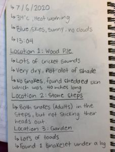
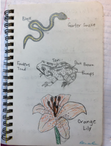
The organisms I’ve chosen to study are the garter snakes (Thamnophis sirtalis).
The three areas I’ve selected area: the wood pile, the stone stairs, and the garden. Today the snakes are staying inside the cracks in the stone steps, this is a good place for them to be today since they’re out of the sun and the temperature is much cooler than the wood pile or garden. This distribution is different from the usual as the snakes are usually found in the wood pile or garden, most likely because there is an abundance of food (insects, small rodents, toads, etc) in these areas.
I think the reason for the snakes staying inside the stone steps today is due to the heat warning. Snakes are classified into the thermoregulating type ectotherms. Meaning that they cannot regulate their body temperatures and therefore must rely on external sources of heat. If a snake’s body temperature gets too high (or low) they can die, to ensure that the snakes keep a suitable body temperature they find cooler places such as the cracks in the stone steps. My hypothesis is that when the ambient temperature reaches over 30*c the snakes will spend the day in the stone steps.
My predictions are that the snakes will not be out in the open during hot days and will be together, to conserve body heat, during thunderstorms and colder days. The response variable is the garter snakes, and the explanatory variable is the ambient temperature.
I chose the haphazard sampling strategy because the shorelines of Nita lake varies significantly in vegetation abundance as a result of some particularly steep and rocky areas. In order to determine whether elevation from the waterline (flood prevalence) has a relationship with species composition, I needed to sample areas that had sufficient abundance in vegetation and a gradual enough gradient. The results in my first assignment submission are from Site 2, which is one of four sample plots i chose along the shoreline. I am aware that by subjectively selecting sample sites i run the risk of subconsciously tailoring the results to fit my hypothesis, and neglecting other factors aside from elevation that may have an impact on species composition, such as substrate. I analyzed and recorded the substrates in results, and there appeared to be some correlation between substrate type and species composition, particularly in the higher, less flood vulnerable zones.
I had predicted that Alnus rubra would be the overwhelmingly dominant species in the sub-2 meter elevation zones, as this would align with my hypothesis that Alnus rubra will be the dominant tree species of flood prone areas on Nita Lake. My results demonstrated this, with Alnus rubra composing 100% of individuals in the sub 1 meter zone and 95% in the 1-2 meter elevation zone. However, i was surprised to see that this trend in species composition continued past the flood prevalent zones, with Alnus rubra comprising 89% of individuals in the 2-3 meter zone. The variable that stood out to me in this zone was substrate, with Alnus rubra only growing in the areas with deeper soil, in contrast to the two Western red cedars growing in a thin layer of soil over large rock slabs. This made me give more consideration to the impact of substrate, as well as flood disturbance, on the distribution of Alnus rubra, and the colonizing behavior of Alnus rubra in non flood disturbed regions.
This sampling exercise was my first attempt at practicing my elevation calculation methods. I lodged an upright pole (using a level) in the mud at the waters edge, with markings from 0cm (at the waterline) up to 1 meter height on the pole. I had a string attached to the pole at the 1m elevation mark that, with a helper, i ran horizontally across to where it met the rising slope of the shore line, and attached it to the ground with a tent peg. I used a level to make the string horizontal. This gave me the 1 meter elevation mark in my sample plot. I then lodged another pole in the ground at the 1 meter mark and went through the same process to make the 2 meter elevation mark. I did this two more times to make the 3 and 4 meter elevation marks. This was a slow and tricky process to begin with, however after finishing the second mark we became much more efficient at it, and i think it provides sufficient accuracy for my purposes. I also used these horizontal string lines to determine the perimeters of my 10 x 10m plot.
I will continue to use the haphazard sampling strategy as i found it to be successful in recording these results.
I used the area based systematic, area based random, and area based haphazard methods to sample the Snyder-Middlesworth Natural Area.
The area based haphazard method had the fastest sampling time at 12 hours and 28 minutes, followed by area based systematic at 12 hours and 46 minutes, and area based random at 12 hours and 52 minutes.
Percentage error for the two most common species:
Eastern Hemlock
Systematic: 8.1%
Random: 5.1%
Haphazard: 1.6
Red Maple
Systematic: 5.8%
Random: 29.7%
Haphazard: 22.6%
Percentage error for the two rarest species:
Striped Maple
Systematic: 100%
Random: 28.6%
Haphazard: 18.9%
White Pine
Systematic: 90%
Random: 48.8%
Haphazard: 98.8
There appears to be a strong correlation between higher species abundance and higher sampling accuracy, with significantly higher percentage error in the sampling of the rarest species than the sampling of the most common species.
For the two most common species i found the systematic sampling strategy to be the most accurate, while for the two rarest species Random sampling was the most accurate. There appeared to be great variation in the accuracy of the three strategies, and there was no overwhelming stand out in terms of accuracy.