Recent Posts

Post 7: Theoretical Perspectives

User:  | Open Learning Faculty Member: 


My research is focused on studying the disturbance gradient of ecotones within anthropogenic and natural disturbance zones. Disturbances zones can be defined by the term ecotone and are typically found throughout residential areas. Ecotones will result in a transitional area between two communities where interspecies competition between early to mid-successional species can flourish. I am studying Himalayan Blackberry (rubus armeniacus) and its effects within the Pacific maritime ecozone, as this Invasive species has become problematic within the Pacific Northwest. Himalayan blackberry has the ability to quickly spread and due to its longevity, early to mid-successional species typical of ecotones have been heavily affected. Climax species are not affected by the plant, but environmental factors like arrested succession can occur where rubus armeniacus is allowed to proliferate.

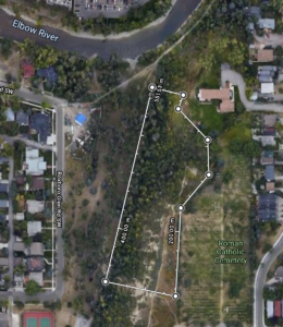
By observing the density and average height over a transect I have been able to see the extent of disturbances and seen how succession has been affected. Structural attributes like biomass will not be included within my report, but I hope to be able to show how functional attributes like productivity, nutrient fluxes, and saturation can affect the growth of the clonal vine. The reduction in biodiversity that Himalayan blackberry has created within the Pacific Northwest has become a problem for land planners and understanding interspecies competition that exists between natives and non-native is paramount to restoring natural ecosystems.

Blog Post 3: Ongoing Field Observations

User:  | Open Learning Faculty Member: 


The biological attribute that I plan to study for my field research project at Erlton/Roxboro Natural Area is soil moisture along a slope. The pattern that led me to this question was the distribution of trees across my gradient. The bottom of the slope was marked by a canopy of large trees, the middle of the slope consisted of frequent, medium-sized trees while the top of the slope was marked by infrequent, notably smaller trees and saplings. I plan to combine these two pieces of information to determine how the angle of the slope impacts soil moisture, and subsequently investigate whether this is a potential limiting factor for tree frequency, and size.

I will conduct my research over the entire area of my slope, but will subdivide it into three horizontal cross sections in order to capture three distinct percent slopes. The first will be just under the top of the ridge on the steepest part of the slope, another will be at the midpoint where it is more moderate and the last one will be at the bottom where the earth is essentially flat (see attached scan below).

Blog Post 3

I hypothesize that slope will impact soil moisture levels and I predict that soil moisture will be negatively correlated with percent slope and positively correlated with tree frequency and size. Furthermore, I predict that there will be a trade-off between tree frequency and size and that as soil moisture reaches it’s maximum, tree frequency will decrease while size increases.


Potential Response Variable: Soil moisture level (instrument specific – could be either)

Potential Explanatory Variable: Percent slope (continuous)


Potential Response Variable: Tree frequency (continuous) and/or size (continuous)

Potential Explanatory Variable: Soil moisture level (instrument specific – could be either)

Blog Post 4: Sampling Strategies

User:  | Open Learning Faculty Member: 


I conducted area-based systematic, random and haphazard sampling methods on the Snyder-Middleswarth Natural Area in the virtual sampling tutorial. Eastern Hemlock (EH) and Sweet Birch (SB) were the most common species found in my simulation, while Striped Maple (SM) and White Pine (WP) were the rarest.

Systematic sampling was performed on 25 quadrats over an estimated duration of 12hrs37mins. The percent errors for EH, SB, SM and WP were 11.47%, 21.70%, 100% and 90.48%, respectively.

Random sampling was performed on 24 quadrats over an estimated duration of 12hrs57mins. The percent errors for EH, SB, SM, and WP were 29.39%, 17.02%, 90.29% and 100%, respectively.

Haphazard, or subjective, sampling was performed on 24 quadrats over an estimated duration of 12hrs40mins. The percent errors for EH, SB, SM and WP were 28.58%, 6.38%, 76% and 197.62%, respectively.

Estimated sampling times were comparable across all three methods; however, systematic sampling had the lowest time and included an additional quadrat, making it the most efficient strategy in this simulation. In terms of accuracy, the margin of error was consistently, and considerably, lower among common tree species (EH & SB) as compared to rare tree species (SM & WP). This finding suggests a decrease in sampling accuracy when dealing with rare tree species.

In this simulation, systematic sampling was the most accurate for two out of the four tree species (EH & WP) and the least accurate for the other two species (SB & SM). Random sampling was never the most accurate method of sampling but it was only the least accurate for EM, by a very small margin (0.81%). Finally, haphazard sampling was the most accurate strategy for two out of the four tree species (SB & SM) and the least accurate method for WP, by a substantial margin (97.62%).

While the results from this simulation are inconclusive, I submit that systematic sampling was the most accurate. It was at par with random sampling for rare tree species, but slightly outperformed it when sampling common tree species. Furthermore, while haphazard sampling yielded the lowest result among the findings (6.38% error for SB), this sampling technique generally yielded inconsistent results. Increasing sample size in future simulations would improve accuracy across all three sampling methods.


Blog Post #3

User:  | Open Learning Faculty Member: 


I have decided to study vegetation abundance with increasing distance from the creek.

  • Cows Parsnip (Heracleum umbellifers)
  • Sweet Clover (Melilotus officinalis)
  • tufted vetch (Vicia cracca)
  • White Clover (Trifolium repens)
  • grasses

I choose four spots along the creek to observe the plants growing there and noticed that wherever the Cows Parsnip was growing, no other plants (besides grass) were growing. The other wildflowers grew everywhere on top of the creek bank, but not near the water. The Cows Parsnip seemed to grow closer to the creek and in damper areas. They also grew more in the shade, while the other wildflowers appeared to grow where there was more sun.


  1. Near Greenhouse.

The wildflowers only grew on the banks of the creeks. The banks here are very steep and the only organism growing near the water is grass. Wildflowers are covering the field next to the walking trail.

2. Near Library.

I stopped seeing the other wildflowers when the Cows Parsnip begins to show up. There is a group of approximately 20 of them in this area. They are in the tall, damp grass and under the shade of the tress. The banks are more shallow here so the other wildflowers are growing closer to the creek.

3. Kin Park Bridge.

The Cows Parsnip are flourishing on the shallow decline to the creek. They are about 2-3 meters from the water.  The closer they get to the creek, the larger and more green they are. The other wildflowers stop near the top of the bank.

4. Across from baseball diamond.

There are tons of Cows Parsnip growing here. There are no other wildflowers here. The Parsnip appears to be greener and have whiter flowers closer to the creek.

It seems as if Cows Parnsip is better suited to survive harsher condition than the other wildflowers. They continue to thrive without sunshine and in very damp areas.

Hypothesis:

My hypothesis is that proximity to the creek will effect the variety of plant life growing in the area.

Prediction:

I predict that the Cows Parsnip will survive closer to the creek due to it being more resiliant to harsh conditions, whereas the vegetation that need more specific conditions (sunlight and water) to survive will not. I predict that the as distance from the creek increases, the variety of plantlife will also increase.

A possible response variable is the presence/absence of the types of vegetation (categorical) and a possible explanatory variable is their distance from the creek/shade of trees (continuous).


Scan of field journal:

Scan (dragged) 2

Scan (dragged)

Blog Post 2: Sources of Scientific Information

User:  | Open Learning Faculty Member: 


a) The source I have chosen to evaluate is Herbicide, fertilization, and planting density effects on intensively managed loblolly pine early stand development by authors Gabriel Ferreira, Benjamin Rau and Doug Aubrey.

b) This source is classified as academic, peer-reviewed research material.

c) As per the How to Evaluate Sources of Scientific Information Tutorial in module 1, in order to determine whether a paper is academic or not three criteria must be met. First that the text in question is written by an expert in the field, second that it includes in-text citations and finally that it contains a bibliography. The authors’ affiliations with the University of Georgia and the USGS New England Water Science Center (Ferreira et al. 2020) ensure that the first criteria has been met. Furthermore, in reading through the paper they make use of several in-text citations and include a full bibliography.

In regards to whether the paper is peer-reviewed or not, the authors acknowledge that there were two anonymous reviewers (Ferreira et al. 2020) at the end of the paper in the “Acknowledgements” section. This classifies it as a peer-reviewed paper.

Finally, again as per the How to Evaluate Sources of Scientific Information Tutorial, the inclusion of “Methods” and “Results” sections distinguishes this paper as a research paper.

References

Ferreira G, Rau B, Aubrey D. 2020. Herbicide, fertilization, and planting density effects on intensively managed loblolly pine early stand development [Internet]. [cited 2020 Jul 20]; 472:118206. Available from:https://www-sciencedirect-com.ezproxy.tru.ca/science/article/pii/S0378112720309750#s0100 doi: 10.1016/j.foreco.2020.118206

Tutorial: How to Evaluate Sources of Scientific Information [Internet]. Kamloops, BC: Thompson Rivers University [cited 2020 Jul 20]. Available from: https://barabus.tru.ca/biol3021/evaluating_information.html#1

Blog Post 1: Observations

User:  | Open Learning Faculty Member: 


The area that I have selected for my field research project is the Erlton/Roxboro Natural Area in Calgary, AB (Figure 1). Located in the heart of Calgary, it is designated as a natural park. This designation specifies the importance of maintaining its natural flora and fauna by the city. This area, covering approximately 13,300m², comprises a hill leading to an upper ridge with an elevation change of about 27m.

Figure 1.

Roxboro & Erlton off-leash dog park flanks the base of the hill on the west side and there are two main walking trails. One trail leads up the side and across the upper ridge while the other meanders horizontally across the slope about 50% of the way up. Other nearby features include a children’s playground, tennis courts, a cemetery, the Elbow River and residential communities. As an important side note, the city of Calgary has posted a sign regarding upcoming herbicide application against dandelions and other broad leaf weeds.


I visited the area on 10/07/2020 in summer at 11:15 until 13:00. The weather was 22°C and mostly sunny. On the day I visited, the top of the ridge was bathed in sunlight while the lower half was shaded, primarily due to the canopy of larger trees (Figure 2).

Figure 2.

The forest floor at the bottom of the slope was marked by a labyrinth of fallen logs and grass (Figure 3).

Figure 3.

Further up the hill, the underbrush of the forest was more dense with greater varieties of grass and wildflowers (Figure 4).

Figure 4.

Just before the slope levels out at the top, the incline sharpens and reveals patches where the ground is more eroded (Figure 5).

Figure 5.

The top of the ridge is flat and riddled with wildflowers, grass, shrubs, and trees (Figure 6).

Figure 6.

Another noteworthy feature is a small spring at the midpoint of the slope that trickles down at the southern end.

On this day, I noted a lot of noise emanating from the surrounding streets, playground, dog park and local construction.

Birds were seen primarily throughout the more forested areas both on the ground and in the trees, sometimes feeding on garbage. Bees were seen among the wildflowers, and I also identified what I believe to be bobcat scat. Among the flora and fauna, several species were identifiable including:

Black-billed magpies (Pica hudsonia)

Northern flickers (Colaptes auratus)

Black knot (Apiosporina morbosa) (Figure 7)

Johnson grass (Sorghum halepense)

Siberian peashrub (Caragana arborescens) (Figure 8)

Canadian violet (Viola canadensis)

Figure 7.

Figure 8.


Questions:

  1. Does the amount of time birds spending foraging on the ground differ statistically across varying proximities to anthropogenic related noise?
  2. How significantly does the angle of the slope impact a tree’s seed dispersal radius?
  3. How significantly different is soil moisture retention between steeper vs. flatter sections, and/or sunnier vs. shadier areas? How might this impact biodiversity in those zones?

Sources of Scientific Information re: 16 Oaks Community Garden

User:  | Open Learning Faculty Member: 


The jumping point for establishing a novel insect biodiversity case-study analysis of potential impacts from contaminated soils in an urban community garden ecosystem at 16 Oaks Community Garden comes from a research article published in the Journal of Soil Sciences and Plant Nutrition.

The article in question titled “Soil assessment for urban agriculture: a Vancouver case study” was written by G.A. Oka, a Masters of Science student at the University of British Columbia Soil Science program, coauthored by L. Thomas, and Dr. L.M. Lavkulich, faculty members of the same university in 2014.

Using the assessment matrix, “Tutorial: How to Evaluate Sources of Scientific Information” included in the course materials, the article is considered academic in nature due to field expertise of its main author. This process is further supported by the research articles successful submission for publication in an academic journal. Using in-text citations to establish sources of external information, the article supports its academic purview using a listed reference section at the end of the article publication. However, the article is not refereed and therefore is classified as academic non-peer reviewed article.

G.A. Oka, L. Thomas, L.M. Lavkulich. (2014). Soil assessment for urban agriculture: a Vancouver case study. Journal of Soil Science and Plant Nutrition. 2014, 14 (3), 657-669. http://dx.doi.org/10.4067/S0718-95162014005000052

Post 4: Sampling Strategies

User:  | Open Learning Faculty Member: 


  Systematic  Random  Haphazard 
Fastest estimated sampling time  12 hrs 38 mins  12 hrs 45 mins  12 hrs 30 mins 
Percentage error Eastern Hemlock   

((520-469.9)/469.9)) *100 

10.7% 


((479.2-469.9)/469.9)) *100 

1.98% 

((583.3-469.9)/469.9)) *100 

24.1% 

Percentage error Sweet Birch   

((124-117.5)/117.5)) *100 

5.5% 


((120.8-117.5)/117.5)) *100 

2.8% 

((166.7-117.5)/117.5)) *100 

41.9% 

Percentage error Striped Maple  ((0-17.5)/17.5)) *100 

100% 


((12.5-17.5)/17.5)) *100 

-28.6% 


((20.8-17.5)/17.5)) *100 

18.9% 

Percentage error White Pine   

((4-8.4)/8.4)) *100 

-52.4% 


((0.0-8.4)/8.4)) *100 

-100% 

((20.8-8.4)/8.4)) *100 

147.6% 

Accuracy  Moderate accuracy for common species 

Poor accuracy for least common species 


High accuracy for common species 

Poor to very poor accuracy for least common species 


Poor accuracy for common species 

Moderate to very poor accuracy for least common species 


Of the three sampling types, haphazard had the fastest sampling time but only marginally. It was 8 minutes faster than systematic sampling and 15 minutes faster than random sampling. I would expect random sampling to have the longest estimated sampling time as this can be a difficult method to carry out under field conditions. None of these estimated sampling times would give me enough information to choose which sampling method would be appropriate for a given project to reduce time costs. Possibly with a larger sample size (>24) the estimated sampling times would show greater variance amongst the sampling methods, providing better information to make a decision for project cost. 

To calculate percentage error, I based this calculation on the information provided for density (not frequency or dominance). The percentage error for the two most common species (Eastern hemlock & sweet birch), haphazard had the highest percentage error for the sampling method. This is to be expected because the plant community is more heterogeneous which tends to offer more biased, unrepresentative estimates. Random sampling offers reliable estimates with the least amount of bias and as a result, had the smallest percentage error for the two most common species. 

The two least common species had large variations in accuracy of density. The percentage error for density may be showing such variations as White Pine and Striped Maple are typically small species in terms of basal area (or diameter at breast height). This would cause a disproportionate representation of density and it may have been a better idea to calculate percentage error on dominance and not density. Dominance provides the total basal area of a given species within the unit area of the community. 

Species abundance does not appear to heavily influence percentage error accuracy in my findings, it only affects the result from overestimates and underestimates. Possibly with a larger sample size, this error would be greatly reduced. Using a species-area graph would have helped with sample size, ensuring that species richness is represented but once the graph starts to level off (no more addition of new species) no more additional samples are needed. 

Random sampling had the greatest time estimate but it also had the highest accuracy for the density of common species. I also appreciate the lack of bias in this method and would tend toward this sampling method. 


Blog 3: Ongoing Field Observations Lost Lake

User:  | Open Learning Faculty Member: 


PROCESS 

Each visit I had to my chosen site left me wondering what attribute to study. At a certain point, I thought that identifying mosses and their location based on limiting physical factors of water availability would be a great way to increase my abilities to identify mosses. However, I couldn’t define a pattern – just that moss grows everywhere around Lost Lake, including underwater. I also want to make sure that I stay on the trail system as much as possible to avoid damaging undergrowth or acting contrary to park rules. I am in a populated area and my actions may be copied by a park user unknowingly.  

The next organism that I noticed, are conks! I am only seeing the conks growing in one stand of trees on the west side of the lake in a square area of about 25 m2. This is now the organism I have decided to study as I noted its presence heavily on the west side of Lost Lake but nowhere else around the Lake.  

HYPOTHESIS 

The distribution of conks growing on trees at Lost Lake is limited to tree species and is determined by tree health.  

PREDICTIONS 

I predict I will find conks growing on only one tree species in all sections of the tree (lower third, mid-third and top-third) and that I will find conks on trees that have obvious signs of health decline (diminishing canopy, excavation by wildlife, browning needles, severe lean). 

POTENTIAL RESPONSE AND EXPLANATORY VARIABLES 

My predictor variable is tree species (type). My response variables are the conks (presence or absence) and tree health (good or declining). Both the predictor and response variables are categorical as they are classified into one or more unique categories. 


Blog Post 6: Data Collection

User:  | Open Learning Faculty Member: 


I have completed my data collection. In total, I chose 15- 1 m squared replicates within each of my 16 transect lines. I intend to capture the spatial coverage of Himalayan Blackberry (Rubus armeniacus) in differing ecotone environments around my neighbourhood. I did this by measuring height and density (cover class).

My data collection went well, although it was hard to access some of my transect locations due to the bushes being un-passable. I had long pants on and big boots, then I paced one large step for every meter and would record relevant information. Areas where I could not access I would estimate height and location within the transect. I was hoping that by doing 15 – 1 m squared quadrats being slightly wrong on exact location would not influence my results too greatly, as I would still capture the general variability. I also did this in one day so growing patterns would not influence my results

I am starting to realize that Himalayan blackberry is opportunistic. I believe I am going to be able to disprove my hypothesis. Instead of preferring ecotone environments, the Himalayan Blackberry seems to be opportunistic appearing in most transitional locations.