Recent Posts

Blog Post 6: Data Collection

User:  | Open Learning Faculty Member: 


Thus far, I have been able to identify shorebirds (to measure shorebird diversity) at 5 sampling quadrats at each location along the human presence gradient (gradient comprises three different sampling locations) 6 times. Hence, I have collected 30 replicates for each location along the gradient. I haven’t had any problems implementing my sampling design so far, except for the fact that it requires a lot of planning in regard to timing in attempt to control for timing variations of shorebird diversity. Thus far, it seems like shorebird species richness, evenness and abundance decreases across the sampling gradient. However, I would still like to collect more replicates for each location along the gradient to see if this effect persists with more samples collected.

Post 3: Ongoing Field Observations

User:  | Open Learning Faculty Member: 


With my next visit to Heritage Park I looked toward the stream located on the west side down from the gravel walking path. I’ve decided to study how the plant community changes along the riparian stream side as proximity to the stream changes. I want to know if these changes also occur with increasing changes in elevation.

I began my observations at the lowest point of the stream that I could access before there is a sudden drop into a ravine. Here the stream forms a small pond near a walking bridge. I took note of the vegetation in three rough points: near the stream, mid point up the bank and the upper portion of the bank near the gravel path.

I did the same at a second site near a bubbling pipe that allows water to flow through an area with a small dam, and then again once more further upstream.

My observations seem to indicate, for one, that the type of flora along the riparian bank seems to be more influenced by other factors than just the presence of the stream itself, but that there is a slight increase in plant diversity as proximity to the stream decreased. Some species known for their preference of moist soils such as salmon berry (Rubus Specabilis) were often present with few others such as fern species near the water, with the exception of the first site which also had some ground cover plants mixed in as well. Further back up the bank I found species such as black hawthorn (Crataegus douglasii) and other tree and shrub species mixed in with Himalayan blackberry (Rubus armeniacus) as well as other invasive species such as creeping buttercup (Rananculus repens). It seemed there was more diversity of species the farther away from the stream I observed. How far does this diversity go? Is there an average to the maximum amount of diversity before the level drops again?

Hypothesis – Proximity to the stream affects plant diversity at Heritage Park

Prediction – Plant diversity increases with an increase in elevation away from the stream. There is a maximum to this however before diversity averages, then drops.

Response variable – Number of plant species present (Continuous)

Explanatory variable – Distance from the stream (Continuous)


Post 2: Source of Scientific Information

User:  | Open Learning Faculty Member: 


a) For my scientific information source, I chose the following academic manuscript discussing the variations of Populous trees of riparian zones of Alberta which is a big portion of my site observations:

Floate, K. D. (2004). Extent and patterns of hybridization among the three species of Populus trees that constitute the riparian forest of southern Alberta, Canada. Canadian Journal of Botany. NRC Canada. 82:253–264. doi: 10.1139/B03-135.

b) This scientific paper is an academic peer-reviewed research manuscript. This publication indicates that the author is affiliated with a University and is an expert in his field at the Lethbridge Research Centre. His article has in-text citations, has a reference page, methods and results.

c) The Canadian journal of Botany demand that every piece of literature is refereed prior to publication.

“The Canadian Journal of Botany (Can. J. Bot.) is a refereed, primary research journal that publishes Articles, Notes, Commentaries, and Reviews, in English or French.”

Source: Instructions to Authors. (2001). Canadian Journal of Botany. National Research Council Research Press. 79(1). https://doi.org/10.1139/cjb_instruct01_e

And finally, the amount of time it took to get to publication.

“Received 6 May 2003. Published on the NRC Research Press Website at http://canjbot.nrc.ca on 15 March 2004.”

Blog 1: Observations

User:  | Open Learning Faculty Member: 


My chosen study area will consist of observing a varied riparian zone along the Highwood River, southwest of the town of High River, Alberta. This location is just 300 meters south of my house and has suffered major damages from the 2013 floods. The Highwood river originates from the collection of water from the slopes of Mount Arethusa, flowing southeast towards the Bow River. This study area is surrounded by cultivated, pasture and rangelands with pockets of native grasses. I have decided to divide approximately a 1km area into three sections due to its contrasting ecosystems.

In plot 1 I am observing 80 meters of a 150 meter section of sandstone plateau caused by old erosion (pre flood) exposing various sedimentary layers where moss, shrubs, flowers and grassy vegetation is sparsely growing across the northern rocky slope just below a 4ft bank housing old swallow cavity nests.
Plot 2 spans approximately 700 meters east into a old growth forest with a gentle slope till it reaches river elevation. Black cottonwood (Populus trichocarpa), Balsam poplars (Populus balsamifera) and hybrids are to be identified once the trees leaf out. Various shrubs and plant life fill the forest floor from short grasses to tall, willows and flowers. This area has massive debris piles and downed trees and river rock spread at least 200 meters from the river edge.
My last plot is a wetland section roughly 150 meters from the river edge spanning 500 meters east, tucked below an old cut bank of approximately 9 feet behind the house of our neighbour. These are 3 fluctuating hydroperiods which were influenced by the change in topography from the floods.

My initial observations started on May 07, 2020 at 10:30 and ended approximately at 13:00 hour on an overcast day, with winds ranging from 2-8 km/hr on average. Because of the late spring, my observations lack identification of flora mostly due to the phenological timing. However, we are in the middle of bird migration and some are already having territorial disputes, are mating and collecting nesting material. Tracks and scat were also noted (ungulates, canids, lagomorphs, rodents).

Questions:

How old on average are the trees in this riparian zone? Can I identify if cottonwood types (black or plains), balsam poplar (Populus balsamifera) or hybrids dominate the area?

Does the vegetation differ in each plot? does the pattern and communities change with environmental gradient? What are the succession stages in each plot?
What are the native species, invasive species and introduced species? Which ones are thriving? Is there a different pattern in each plot? Are soil types and recent processes big factors for community diversity and distribution?

What are the main ecosystem disturbances in each plot? Which one has greater chances of thriving despite the disturbances?

Which plot is most attractive for fauna diversity? How important are riparian zones for wildlife? Are riparian zone processes and successional events too volatile for specie site fidelity?

Blog Post 4: Sampling Strategies

User:  | Open Learning Faculty Member: 


My results for the simulated forest sampling are below. While the haphazard technique was the fastest, it’s overall accuracy as abysmal. I found it interesting that for the most common and least common species, the random sample was the actually the most accurate, while the systematic approach was the most accurate for both the second most common and second least common methods. With the systematic approach, the accuracy dropped as the species became less common. As mentioned, this didn’t prove true with the random sample however, which was a lot more random in its results as it’s nature would suggest.

In conclusion a systematic sampling approach in this setting may work the best if you know your target species is fairly common while a random approach may be the best method if you are unsure. Based on this experiment I would definitely try to avoid haphazard sampling if it can be avoided.

Systematic Area Based  –

Easter Hemlock – Actual – 469.9  Estimated – 524   Error –  12%

Sweet Birch – Actual – 117.5 Estimated – 136  Error –   16 %

Stripped Maple – Actual – 17.5 Estimated – 12  Error –   31 %

White Pine – Actual – 8.4 Estimated – 12  Error –   43%


Random –

Easter Hemlock – Actual – 469.9 Estimated – 487.5  Error –   4 %

Sweet Birch – Actual – 117.5 Estimated – 137.5  Error –   17%

Stripped Maple – Actual – 17.5 Estimated – 0  Error –   100 %

White Pine – Actual – 8.4 Estimated – 8.3  Error –   1 %


Haphazard

Easter Hemlock – Actual – 469.9 Estimated – 579.2  Error – 23%

Sweet Birch – Actual – 117.5 Estimated – 275  Error –   134%

Stripped Maple – Actual – 17.5 Estimated – 29.2  Error –   66 %

White Pine – Actual – 8.4 Estimated – 20.8  Error –   147 %


Post 2: Sources of Scientific Information

User:  | Open Learning Faculty Member: 


I’ve chosen a book entitled “Edible and Medicinal Plants of Canada” by Andy Mackinnon, Linda Kershaw, John Arnason, Patrick Owen, Amanda Karst and Fiona Chambers to use as an ecological reference. This book focuses on the uses of plants, which is of personal interest, but more importantly from an ecological standpoint, has detailed descriptions of the plants, their flowers and fruit as well as where they grow, including moisture preferences and soil type. The book contains references, and the authors are assumed experts that are well decorated with degrees and experience. Based on what we have learned about classifying scientific information, I would classify this book as being a non-peer reviewed academic material.


MacKinnon, A., Kershaw, L., Arnason, J., Owen, P., Karst, A., & Hamersley Chambers, F. (2009). Edible and Medicinal Plants of Canada. Edmonton , Canada: Lone Pine Publishing .

Post 1: Observations

User:  | Open Learning Faculty Member: 


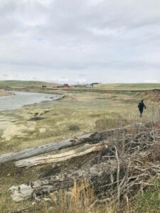
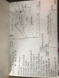
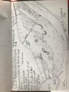
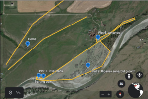
The area I’ve chosen to observe is Heritage Park in Mission, BC. This is a city park with an area that is approximately 1.6 square km. When entering from the West side there is a large grassy hill that descends into a forested which then drops into a small stream that flows from the north. From here there are several forested hills, but a general increase in elevation as you move north and east.  This forested area is home to a network of hiking trails.

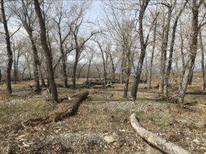
Today was sunny and 15 degrees when I visited at 16:45. I observed several plant communities and tried to take notice of changes that occurred where several gradients met. For example when the grassy hill met the forest it was surrounded by Himalayan blackberry immediately near the path but behind that at the hill descended further existed a more natural community of big leaf maples with an under story of vinemaple while sword ferns and pacific bleeding heart acted as a ground cover. I walked down the path and noticed a different community just to the west where small patch of forest existed. Here I observed a stand of alders as the canopy, with vine maples and swords ferns below. Here however there were also deer ferns. What made this section home to alder instead of big leaf maple, and what why did deer fern exist here, while only sword fern existed on the slope less than 10 meters away on the other side of the path?

As I followed the path northward, I noticed many invasive species on either side. Buttercups, broadleaf plantains, dandelions, small patches of the non native stinging nettle and some himalayan blackberry. There was far less of the blackberry here however, why was that? How far do the invasive plants grow off the path? How do their communities change with elevation? Is there a relationship between where a particular native species grows and where the invasive plants are stopped?

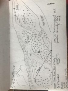
I also noticed a change in the plant life as I climbed slightly in elevation. More thimbleberries in denser patches, a few cedars began to dot the landscape, some huckleberry bushes here and there. In certain places salmon berry became the main understory shrub.

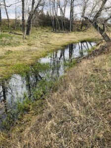
I came to a place where a small path led off the gravel and down toward the stream. I followed this to the stream and when looking back I could see some obvious changes in the plant life as the path descended toward the stream. Up near the gravelled path existed thimbleberry, a cedar and a struggling alder sapling. As the elevation dropped toward the water, there grew a thicket of salmonberry under a bigleaf maple and a vinemaple growing at it’s side. Are these changes due to the elevation, the disturbance of the gravel path or simply the water source? Do similar changes in plant communities exist near other streams in the park?

Beyond the questions I’ve already asked while visiting the site a few others that may make for interesting research include: How does the the relationships of particular plant and tree species change with elevation, distance from the disturbed hiking trails, or near a water source? I noticed there weren’t many birds here, does this change with plant communities, elevation or time of day? Is there variation in flowering between different blackberry, thimbleberry or salmonberry thickets? If so, why could that be?

Blog Post 8: Tables and Graphs

User:  | Open Learning Faculty Member: 


Getting Microsoft Excel to put all the data I wanted into the graph in a logical way was extremely frustrating. I was not aware that it would be so complicated to format the spreadsheet properly in order to get the proper variables on the proper axes and the right data to be represented by multiple lines. Once I figured out the formatting and how to edit every single piece of the graph to be the right colour and the right line thickness, everything went well. I found that using the combination graph with three axes with different scales was actually not as simple as rearranging the data and using the scatterplot statistical graph for the two quantitative variables. Within this format I could embed two data sets on two lines to compare them in one graph instead of two separate ones, and I could then label the points and lines appropriately within the actual graph or using a legend. I wish there was a way to set a template with all the colours, data point symbols and line designs, so that every time I made a graph I didn’t have to go and change 20 different things in order to make it all look right. I also wish I had the money to pay for Adobe Pro so that I could put the graphs wherever the heck I wanted in my report and wasn’t subject to Microsoft Word’s authoritarian layout rules.

I found some interesting things when plotting the data, but it largely reflected my predictions and hypotheses. When I plotted the data in box plots to identify outliers it largely made up for any discrepancies in the patterns of my original data. I did not expect the elk or deer scat density to be so low in the riparian zone, nor did I expect the deer scat density to be so high in the forest. If I could, I would set up game cameras and see what the animals are up to and how often the deer actually do use the riparian zone. It’s quite obvious from the presence of deer tracks that they are using the riparian area, but for some reason their scat is almost absent. It’s possible the ground is so wet it dissolves, or is engulfed by the muck over time, or maybe they just quickly move through the area to access other feeding areas. One thing that would be worth investigating is whether elk are actually using this area on a yearly basis. If they are, they must cross the Island Highway in order to do so which poses a risk to human and animal life. If there was a way to increase their habitat on the other side of the highway and deter them from crossing into town just to spend a small fraction of time in this small area, then it may be wise to do so.

Blog Post 7: Theoretical Perspectives

User:  | Open Learning Faculty Member: 


My research focuses on two ungulate species: the Columbia black-tailed deer and the Roosevelt Elk. Underlying my  research into their scat densities and their relationship with differing dominant vegetation, is how these two species have adapted to resource partitioning within their similar niches. I look to touch on how nutritional availability changes throughout the year within the plant cells of their preferred food, as well as their differing nutritional needs. I also look to explore how not only nutrition but also predation affects their behaviour in choosing habitats, as well as how this predator pressure may influence their fitness. The understory of the forest in coastal BC is dense with fern, salal and huckleberry which give deer a year round source of food and cover, but during the winter they must share this habitat with the elk.  In spring and summer the elk tend to stick to meadows to eat grasses and sedges and are constantly migrating in order to sustain their nutritional needs. Deer also venture out into the open to use these areas mostly under the cover of darkness when predators are present in the environment. I am looking to investigate to what extent the elk use the grassy riparian areas opposed to the forest, and to what extent black tailed deer share this habitat and the forest with them.
The conservation of the Roosevelt elk populations on Vancouver Island is of great importance to not only the biodiversity of BC but also for ecological stability, anthropogenic economic benefit, and indigenous cultural importance. The preservation or creation of habitat is not only the responsibility of the province but also the forestry industry. More research should be done to see if seral stages or alternative stable states that would increase elk habitat could be allowed to develop by forgoing the application of silvicultural methods that suppress important food sources.

Keywords: Resource partitioning, niche breadth, competition, diet diversity, seral stages.

Blog Post 4: Sampling Strategies

User:  | Open Learning Faculty Member: 


The method I chose for the virtual forests tutorial was the area based method. The fastest sampling method was the systematic sampling method with a time of 12 hours 37 minutes, which was actually only within 20 minutes of the other methods. For the two most common species the systematic was the most accurate and was within a -7.2%  and 5.5% sampling error, compared to 63.4% and 100.9% error for the haphazard, and 11.2% and-29% error for the random method. For the rare species the haphazard sampling method was the most accurate of the three methods, although it still had a 52.4% error for the white pine and -8.5% for the Striped Maple. The random sampling method gave an almost 200% error for the White Pine and a 100% error for the Striped Maple, and the systematic sampling method gave a 174% and -100% error for the Striped Maple and White Pine respectively.

In general the accuracy declined with both the systematic and random methods as the species got more rare, and slightly increased in accuracy for the haphazard method for rare species. The Shannon-Weiner diversity was calculated to be the identical for the true diversity and the systematic method which leads me to believe that it was the most accurate method, along with having lower percentage error for most species present. For the random and haphazard methods the diversity was found to be 1.4 which is 0.1 lower than the true diversity. I don’t believe there was enough points to capture the diversity of species because in both the systematic and the random methods, one species was not observed at all. Even though the Shannon-Weiner diversity was found to be accurate for the systematic sampling method, I would consider increasing the number of samples in order to guard against inaccuracy.