Recent Posts

Post 8: Tables and Graphs

User:  | Open Learning Faculty Member: 


I had a hard time inserting my data onto a graph as my numbers were a little strange and I had multiple data points with the same x and y-value. I initially thought I would use a scatter plot but after trying that in Excel, I realized it looked quite messy and the data was difficult to understand. So I decided the best way to illustrate the patterns in my data would be two bar graphs that show the means of soil moisture and the means of number of ferns for each transect. I felt the trends in my data were much easier to understand this way. Although I only submitted the bar graphs figure for Small Assignment 5, I think I may also use a table in my paper to insert the specific data from each quadrat.

Based on my bar graphs, I could clearly see that both Transect A and C had similar levels of soil moisture, but Transect A has a much higher number of ferns than Transect C. Furthermore, although Transect B was the most dry, it had a similar number of ferns to Transect C. This outcome is not what I expected as I had hypothesized that as soil moisture increases, the number of ferns would also increase. I will have to consider other factors that may contribute to this pattern while writing my paper, including shade, degree of slope, and soil pH.
Post 7: Theoretical Perspectives

User:  | Open Learning Faculty Member: 


My study investigates the effect of soil moisture on Polystichum munitum abundance along a slope gradient. After collecting my data, I realized that my hypothesis was wrong so while my main focus is soil moisture, I will also have to take into consideration how other factors such as slope and canopy cover affect both soil moisture and fern abundance. It’s important to understand that species growth and abundance is dependent on a number of different factors. Some other ecological influences that I might briefly touch on in my paper and that underpin my research are soil pH, soil nutrition, interspecies competition, and disease. Therefore, my study would fall under a form of population ecology that focuses on how both abiotic and biotic factors affect a species or organism.

My keywords are the following: Polystichum munitum, soil moisture, slope gradient 

Post 6: Data Collection

User:  | Open Learning Faculty Member: 


My data collection went quite well. Soil moisture can be affected by rainfall so I had to make sure I completed my data collection at one time. I collected my data on May 28th at around 1pm PST. It was a cloudy day, but it had rained quite a bit the day prior. I used pre-measured string to establish three transects about 10 m apart from each. One was along the top of the upper-slope, one in the middle, and one along the creek at the bottom. I placed five 16m2 quadrats on each transect, 4 meters apart from each other. This gave me a total of 15 replicates. 

The biggest struggle I encountered was that the rain from the previous day had made the slope quite muddy and slippery. This made it especially difficult for me to place my quadrats and transect in the middle of the slope. I slipped a few times and got mud all over me. Another small difficulty was the insertion of the soil moisture meter. At some quadrats, I really had to push hard to get the meter all the way into the soil to the marker. 

A pattern I noticed was that the soil moisture was around the same at both the top and bottom of the slope. However, the number of ferns was a lot more abundant at the top than at the bottom. This does not align with my hypothesis and I will have to reflect on some other factors on why this could be while writing my paper. I will take into consideration the greater shade at the top, as well as the bottom of the slope not being drained enough for ferns to grow. 

Blog Post 5 – Design Reflections

User:  | Open Learning Faculty Member: 


The most challenging part of implementing my sampling strategy was spacing my sampling sites appropriately so they maintained independence. Although I would have liked to have included more sampling sites, it was not feasible given the limited area of the shrub habitat type. This has also made randomization challenging, although I have introduced it by randomizing which site is sampled first during each survey round. So far, the data I have collected has not been overly surprising. Bird species which are more associated with forest habitat, such as Townsend’s warbler (Setophaga townsendii) and red-breasted nuthatch (Sitta canadensis), have not been recorded within the shrub habitat sampling sites. I plan to continue collecting my data using the breeding bird point count methodology.

Percy Herbert, Blog Post 8: Tables and Graphs

User:  | Open Learning Faculty Member: 


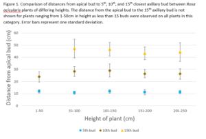
I have collected all of the data for my study on wild rose axillary bud spacing. I generated a figure for Small Assignment 5 to visualize key data. This figure displays plant height (the predictor variable) on the x-axis and the distance from the apical bud to the axillary buds (response variable) on the y-axis.

I originally had planned to show the distances for all 15 buds in the figure for each plant height category. I discovered that when all of this data was included the figure was messy and hard to interpret. By reducing the number of buds displayed to 3 (the 5th, 10th and 15th bud) visualization of the data points and error bars in clear. The inclusion of the data from the 5th, 10th, and 15th bud is a good representation of the full dateset and is sufficient to provide an appropriate visualization. The data from the other buds not represented in this figure may be displayed in a table in the report.

The creation of the figure provides supportive evidence for the prediction that axillary bud spacing is consistent regardless of plant height. The figure shows that at the 5th, 10th, and 15th axillary bud, the distance from the apical bud is easily within one standard deviation for all plant heights and no clear trends are displayed. These results suggest that there is an optimal spacing between the axillary buds for wild roses. For future research it would be worthwhile to further investigate what features have been optimized in wild rose crown architecture and what factors influence these features. For example I would like to investigate leaf size and location to measure the extent of self shading.

Percy Herbert Blog Post 7: Theoretical Perspectives

User:  | Open Learning Faculty Member: 


My research project is an observation of vegetative bud spacing in wild roses (Rosa acicularis).My hypothesis is that the physical spacing between vegetative buds on Rosa acicularis at the Queen Elizabeth Park duck pond is unrelated to the height of the individual plants. My prediction is that spacing of vegetative buds will be consistent for individual Rosa acicularis plants of all heights. I believe that this will be the case as I believe there is an ideal spacing between the buds as to maximize the amount of sunlight exposure to leaves. I predict tall plants will have vegetative buds in the same density as shorter plants as all plants will follow the same ideal spacing at their highest regions to maximize sunlight capture. The optimal vegetative bud spacing should be determined by maximizing leaf surface area at the highest regions of the stem while limiting self-shading. Plants must balance the above factors with the energy cost of producing supporting branches to most efficiently use carbon resources to position foliage in a process referred to as crown architecture.

Key Words: Self-shading, Light Capture, Crown architecture

Post 5: Design Reflections

User:  | Open Learning Faculty Member: 


I collected my initial data on May 20th, 2021 around 1:15pm. I decided on using quadrats along transects for my study. I brought with me a pre-measured 36m string, four 4m strings, and a soil moisture meter. There is a trail that goes along the top of the bank, which is where I chose to place the transect. I used a random number generator to choose the number of footsteps I would take from the entrance of the trail and placed the 36m string there, along the top of the bank. I placed my quadrats along the transect about 4m from each other and collected my data. I used the soil moisture meter directly in the centre of the quadrat to measure how moist the soil was and then I counted how many ferns were in that quadrat. In order for a fern to be counted, more than 50% of its total size had to be within the quadrat.

One of the struggles I had was that the bank was quite steep at some parts which made it difficult to place the quadrats safely. I was afraid I would slip and hurt myself. I think I might bring somebody with me to help me navigate the terrain safely next time. I also realized later that I should have made sure that the soil moisture meter was inserted into the soil at the same depth in every quadrat in order to reduce any inaccuracies in the moisture readings. I will mark the meter with a Sharpie next time and make sure I push the meter up to that point during each of the readings. Overall, I was quite happy with my study design as it is not overly difficult for me to conduct and is very interesting.

I did realize I will have to revise my predictions about my hypothesis. I had originally predicted that as soil moisture increases, fern abundance would decrease. However, after also choosing a quadrat by the creek that had a lower soil moisture level and observing a lower number of ferns, I will now predict that as soil moisture increases, fern abundance also increases.

Blog Post 5: Design Reflections

User:  | Open Learning Faculty Member: 


The hypothesis for my research project is the length of time a Robin spends foraging in the meadow will differ from in the dog park. I predicted that the length of time a Robin spends foraging in the meadow location will be greater than in the dog park location due to the greater number of dogs present within the dog park than the meadow. The sampling method I have chosen will be the Point Count method. I visited the Meadow 5 times, approximately the same time between 5:00-7:00 PM and observed the Robins in the meadow for 30 minutes on May 3, 4, 5, 7 and 8, 2021. The sampling strategy was relatively simple. I sat at a picnic bench with my binoculars and timed the presence or absence of Robins foraging. Considering the time of day, I was surprised by the number of Robins actively foraging and how easily they would return from the meadow once a dog had left the area. I also observed some competitive behaviour between Robins, which I also thought was very interesting. Given the simplicity and lack of resources available, I have chosen to continue using the same sampling method. 

The excerpt from the field journal can be found here: https://drive.google.com/drive/folders/1xbUUajwJ8BOtYKSs8DY5s1f7doOIsc72?usp=sharing. Observations were recorded on the left-hand pages, including weather and activity within the meadow. The right-hand pages document when the foraging time (FT) began, which is defined when at least one Robin was present in the meadow. The foraging time stopped (FTS) when no Robins were present in the meadow. Time was recorded as minutes and seconds. The number of birds and dogs was recorded during one complete cycle of FT to FTS. The FT would begin again when at least one Robin returned to the vacant meadow. Please refer to table one for a list of acronyms. 

Table 1. List of Acronyms

Acronym

Meaning
FT Forage Time
#B Number of Birds
#D Number of Dogs
FTS

Forage Time Stopped

Untitled

User:  | Open Learning Faculty Member: 


The chosen study area is in my backyard (private property) in the residential neighborhood of Aberdeen in Kamloops, B.C. The surrounding vegetation is ornamental and the topography is rolling hills. My last site visit was on May 23rd 2021 at 11:00am and the weather was sunny (26°C) with no precipitation.

My proposed study is to conduct an experiment that measures the growth rate of sunflower plants based on 2 different watering volume applications (i.e. 2 study groups). The study would be conducted over a 6-week timeframe during the spring/ summer of 2021. This would involve growing potted sunflower plants, side by side, in an area that is approximately 20 m2. Half of the potted sunflowers would receive a consistently higher volume of water applications than the other study group, which would receive a lower volume of water throughout the experiment. There would be a total of 24 sunflower plants used in the experiment. There would be 12 sunflower replicates – in each study group – which would all receive the same watering volume applications. The corresponding plant growth rate would be measured for both study groups. All of the other design variables would be constant (controlled), including the – location, sunlight, growth medium, climatic conditions, and watering application time intervals.

Other potential study subjects include setting up a similar study, as the aforementioned, except with using a different predictor variable, such as:

  • Measuring potted sunflower plant growth rates at 2 different locations (in my backyard) that have different sunlight exposure levels, including – a full shade and a full sun exposure location.
  • Measuring sunflower plant growth rates by comparing the use of fertilizer to unfertilized plants.

Potential study questions, include:

  • Is the sunflower plant growth greater in the high-water volume application study group?
  • Is the sunflower plant growth greater in the full sunlight exposure study group?
  • Is the sunflower plant growth greater in the fertilizer study group?
  • blog 1 photos

Percy Herbert, Blog Post 6: Data Collection

User:  | Open Learning Faculty Member: 


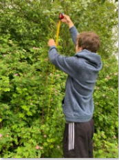
I was able to collect measurements on 50 replicates at the Queen Elizabeth duck pond.  50 individual wild rose plants (Rosa acicularis) were observed. Ten replicates were recorded in each of the five height categories (1-50cm, 51-100cm, 101-150cm, 151-200cm, and 201-250cm). The heights of the plants were recorded as well as the distance from the apical bud to each of the first 15 vegetative buds.

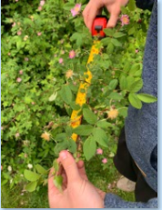
Measurements were much more difficult to collect this time compared to the first data collection as the vegetative buds have all sprouted into small branches containing leaves and flowers. The new growth is all a vibrant green colour while the original stems are a rich red colour so it is still easy to tell the difference between the new growth and the stem. The new growth made seeing the measuring tape and the junctions of the new growth and the stem much harder. Although the measurements were harder to collect, with added time accurate measurements were still possible.


One issue with data collection is that for some of the shorter plants observed there were less than 15 buds. This is especially true for the 1-50cm category. This may lead to the exclusion of this category in some of the data analysis steps.

Initial data analysis appears to support the hypothesis. The spacing between the buds does not seem to be altered by plant height. An ANOVA will have to be conducted to confirm this observation.