Recent Posts

Post 6

User:  | Open Learning Faculty Member: 


Since my last posts, my project has changed substantially.  I am now observing if the presence of red-osier dogwood within 1 meter of conifer tree decreases its chances of being browsed by ungulates.

This was completed at LC Gunn park in Prince George.  I created seven 30 meter transect lines, of which I counted every regenerating conifer stem within 1m on either side of the transect.  I then recorded the height of the tree, if it was browsed by an ungulate, and if red-osier dogwood was present within a 1 meter radius of the tree.

I actually did notice that less regenerating conifers were browsed if red-osier dogwood was present.  However, I am still unsure as to why this is.

Data collection went smoothly, and I did not see any reason to change my methods.  In total, I counted 68 trees, with the majority being subalpine fir, then Douglas-fir, and hybrid spruce, respectively. Of those, 30 had red-osier dogwood present within 1 meter, while 38 did not.

Blog Post 9: Field Research Reflections

User:  | Open Learning Faculty Member: 


Completing my field research and searching through scientific papers for more data confirmed and reinforced what I had just suspected to be the case when it came to completing ‘proper’ science, especially in the outdoor environment rather than in a more controlled environment. My four major takeaways were:

  1. Truly attempting to account for all potential variables in a dynamic environment rather than a lab setting is very time consuming! I found the comments from this blog and my instructor to be very helpful in finding holes that would render my observational results less reliable as well as learning from other field studies I read. In my opinion, from my experience with this small trial in an ecological field study, communicating with other members of the scientific community would be critical in producing good work; sharing information, giving constructive criticism, and accepting criticism.
  2. This field study really helped me understand just how much a research project in the field is a constant work in progress, continually revisiting and adjusting the hypothesis as new variables were recognized or pointed out to me. I believe this may be a taste of what the term “Physics envy” means. It is especially apparent when I think of all the potential anthropogenic influences that may be unaccounted for. I wonder where is the line between time/money accounting for every little variable and it being ‘good enough’ to be accepted as evidence?
  3. The actual physical terrain made me adjust my methods twice. I had to account for the ocean tide so I could actually reach my sample locations, in some areas the slope was too steep to traverse, and in others it was too thick with vegetation to access. I also felt this was a great example of a study that could not be done in any season except the dormant one, as once everything buds out, it would be very difficult to find any Alnus rubra seedlings among the blackberry and rose.
  4. More samples would be better! I’m taking a statistics course as well and feel that the combination of of the two courses made it clear that more samples=more accurate data. Unfortunately due to working full-time and other commitments (not to mention everything is budding out now) I did not generate more replicates to do so.

This project made it very clear to me just how much time (including the researchers personal time!) and money can be required to produce good scientific studies within the field of ecology. This is necessary in order generate honest and reliable evidence that ecological areas need to be preserved, protected, and reestablished where possible, especially in an age where everything is scrutinized so intensively.

The sooner I can get involved the better!

Blog Post 5: Design Reflections

User:  | Open Learning Faculty Member: 


The only difficulty that I had implementing my stratified random sampling technique for identifying shorebirds within each of my specific locations (3 locations along a gradient of human presence) was the fact that I didn’t have a way of measuring a large area to ensure that each quadrat/plot (my sampling unit) could be equal in area. I tried to identify birds within a relatively uniform circumference for my sampling plots/qaudrats. The data I collected was not surprising as it seemed to follow the expected trend of increasing shorebird diversity with a decreasing amount of human presence/urbanization. I plan to use the same sampling approach but I would like to collect more replicate data at various times of day to account for any differences in shorebird diversity across time rather than just space.

Blog Post 8: Tables and Graphs

User:  | Open Learning Faculty Member: 


I had no difficulties in organizing, aggregating or summarizing my data. The outcome was not what I expected. It revealed that there was little correlation between Douglas fir tree abundance and average tree circumference. However, the relationship between tree abundance and aspect of growth was what I expected. The western aspect had the most Douglas fir trees, while the eastern aspect had the least. My data was collected only over the winter season, I would like to explore any changes that may occur in the abundance/circumference and abundance/growth aspect relationships as seasons and weather change.

Blog Post 9 – Field Research Reflections

User:  | Open Learning Faculty Member: 


Blog Post 9 – 03/04/20

Throughout the duration of this course I designed a field experiment that had the objective of determining if soil moisture levels impacted abundance and distribution of three tree species (white spruce (Picea glauca), aspen poplar (Populus tremuloides), and white birch (Betula papyrufera)) in Kinsmen Park. I used a Stratified Random Sampling design to carry out this experiment and overall I felt, upon completion, that the design I chose was well suited to this type of study. Incorporating randomization into the study through selecting various locations to sample from within the designated strata allowed for bias to be completely eliminated. Furthermore, the randomization allowed me to come across some unexpected results that caused me to pause and really reflect upon my hypothesis, the patterns I saw, and the predictions that arose. There were no issues implementing the design. Some days were colder than others, making the ground slightly difficult to sample from, but overall the implementation of the stratified random sampling design went well. Engaging personally in the practice of ecology has certainly deepened and enhanced my appreciation for how ecological theory is developed. My study design was relatively simple and took place over a smaller area. It looked at very simple variables and factors and their impacts on each other. Through conducting my study as well as reviewing previous research for my annotated bibliography, I gained a much deeper appreciation for ecological studies that span years over vast distances and look at multiple variables. The effort that goes into planning and executing these types of studies is immense and the work these researchers are doing to advance ecology is incredibly important. I can’t help but marvel at their dedication to their research, to their field, and to ecology as a whole. Taking this course and performing a field experiment has allowed me to step into the shoes of a ecologist, albeit in a much smaller way, and has allowed me to develop a deepened sense of respect for how ecological theory is developed. 

Blog Post 4 – Sampling Strategies

User:  | Open Learning Faculty Member: 


For the sampling strategy virtual forest tutorial, I selected area-based methods. The most efficient technique in terms of time spent sampling was systemic sampling technique, as it had the fastest estimated sampling time. The systematic strategy was the most accurate sampling strategy for the most common species and the haphazard strategy was most accurate for the least common species. However, the systematic strategy was only the most accurate for the most common species and the haphazard strategy was most accurate for the rest of the species. Accuracy declined as species became less abundant (from common to rare species). Overall, the haphazard strategy was most accurate. The random strategy was the least accurate. I believe that in this case, the haphazard strategy was most accurate because I chose the sampling points within each sampling zone (separated by transects) randomly, so the method that I deployed was similar to the stratified random sampling technique, which is the sampling technique that I will use in my field research.

Blog Post 3 – Ongoing Field Observations

User:  | Open Learning Faculty Member: 


I plan on studying shorebird diversity at the Don Edwards San Francisco Bay National Wildlife Refuge. In particular, I plan on studying shorebird diversity attributes such as species richness, species abundance, species evenness, etc. in response to human presence. In order to study the response of shorebird diversity to human presence at this wildlife refuge, I chose three study locations with varying degrees of human presence across the marsh at the south end of the refuge. A map of the refuge with my chosen study locations are depicted in Figure 1. Location #1 is bordered by a highly urbanized environment, representing the peak of the gradient of human presence. Location #2 relatively closed off from human presence as it is bordered by a wet open grassland which is intersected by a road that leads to the wildlife refuge’s visitor center. This area does not house any trails or walkways and was chosen to represent a minimum of the human presence gradient. Location #3 borders the visiting center and houses walking trails, boarded pathways and bridges for visitors to explore the refuge, observe wildlife, etc.. I assumed that this location would represent an intermediate measure of human presence as this location only houses a visitor’s center and walking trails (minimal urbanization and much less human presence than the urban area bordering location #1). Figure 2 depicts my notes of observed shorebirds in the 3 study locations.

I hypothesize that one underlying process that may be influencing changes in shorebird diversity across a gradient of human presence (or nearby urbanization) may be an intolerance of the local refuge’s shorebird species to urban life or human presence.  Such intolerance may arise from habitat disturbance, pollution, noise, etc.. Based on this hypothesis, I predict that measures of shorebird diversity such as shorebird species richness, species evenness and species abundance should decrease with increases in human presence or urbanization. Specifically, Location #1 (nearby an urbanized environment) should have the least shorebird diversity and Location #2 (little to no human presence) should have the highest measures of shorebird diversity. Furthermore, Location #3 (containing walking trails and human visitors, with little urbanization) should have intermediate measures of shorebird diversity. Based on this hypothesis and predications, one potential response variable would be species richness (a measure of shorebird diversity) which would be a continuous variable. One potential explanatory variable would be the study location which corresponds to particular amount of human presence (Location #1 – high human presence, Location # 2 – little/no human presence, Location #3 – intermediate human presence), which would be a categorical variable.

Figure 1. Map of the Wildlife Refuge at the south end of the San Francisco Bay. The three study locations at which I studied shorebird diversity are depicted by squares (red being location #1, pink location #2 and purple being location #3).


Figure 2. Notes of shorebird observations at 3 study locations along the wildlife refuge south marsh.

Blog Post 9: Field Research Reflections

User:  | Open Learning Faculty Member: 


I appreciate how ecological theory is developed more after conducting my field research. I found it useful to tabulate and interpret the data right after it was collected in the field. I found this useful because it allowed me make changes to the for the upcoming sampling. I also found the preparation of an annotated bibliography very useful for interpreting the results in the discussion.

On the technical side, I had a lot of trouble identifying lichen even after return from the field. I chose the topic initially due to my inherent interest in lichen and background in fungal endophytes, but it presented much more difficult than I imagined. I adapted to this by grouping lichen into the traditional structural categories. This still allowed me to collect data, based on a structure-function relationship with their substrate.

Blog Post 1: Observations

User:  | Open Learning Faculty Member: 


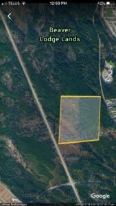
Study area – Beaver Lodge Forest Lands, Campbell River, BC.
Date – March 17, 2020
Time – 13:00 – 16:00
Altitude – 95m
Coordinates 49°58’20 N, 125°15’19 W.
Temperature – 10°C
Weather – sunny, clear skies, no wind
Size of area of interest– Harvested area 0.5km2, second growth forest 0.5km2
Total area of Beaver Lodge Forest Lands – 416 ha

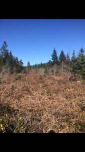
Zone of interest: Transition between the second growth ecosystem and the relatively recent harvested area where no silviculture methods have been applied. Treeline of interest runs North to South. Area is a donated to the province for research in forestry, it is also used for recreation purposes and there is a network of mountain biking and dog walking trails.

Second Growth Ecosystem: Within the canopy of the second growth forest of Douglas Fir, Grand Fir, Red Alder, and Big Leaf Maple, there is evidence of old growth logging (large Western Red Cedar stumps logged by hand with spring board notches still visible). The trees have been planted and the vast majority are Douglas fir and Grand Fir of the same age, though there also seems to be some variation levels of the canopy with young trees growing.  In these areas of disturbance there is new growth of Red Alder and Big Leaf Maple, and in wetter areas it seems Western Red Cedar and Western Hemlock are abundant.

Main Ground Cover: Dominated by Salal, Red Huckleberry, Oregon Grape, Salmonberry, and Bracken Fern, with sparse Trailing Blackberry. The bottoms of the trees were covered in mosses and lichens and there were many areas where trees had blown down opening up the canopy for new growth. Salal and Oregon grape were very green with big broad leaves. Salal leaves were 4” long on average, and Oregon Grape leaves were 3” long on average.

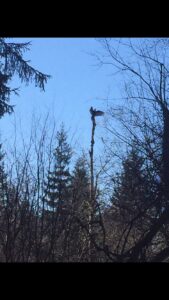
Animals: Not very much Black Tailed Deer sign. Bird life was abundant with American Robins, Varied Thrushes, and Stellar’s Jay flying about. Ravens were observed as well as Great Horned Owl calls (but no sightings this time).

Early Succession ecosystem:
History: Harvested cutblock of unknown age. Stumps are a few years old and it is clear that it was not logged by hand and instead with a feller buncher. It either was hoe chucked or a skidder was used for yarding the logs as machine ruts have overgrown and become water filled depressions. Cleared area is 0.5km2 with a riparian zone cutting through the middle as well as a few small residual patches left standing.

Main ground cover: Bracken fern is dominant in open areas with intense sun along with abundant Red Huckleberry and sparse naturally regenerated Pine trees observed. There is a saturated riparian zone running through the block with slowly running water amongst blue-joint grass, Red Alder, Western Hemlock and Western Red cedar. The ground in this area is completely covered in blue joint grass and moss that seems to have out competed all competition. Salal and Oregon grape are stunted(<0.5m) with smaller leaves (<2”), many are red coloured, Oregon grape only found on the fringe of the forest.

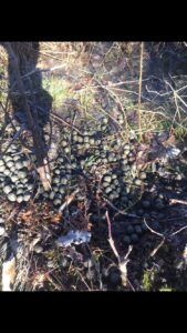
Animals: In the open areas of the cutblock there is a network of Black tailed deer trails with abundant scat and tracks. Some scat old and some more recent (black and shiny). Tracks were observed in the soft soil, measuring 2 ¾“ long, accompanied by much smaller ones which leads me to believe these were from a doe and fawn. In the wet riparian zone with tree cover there is abundant Roosevelt Elk trails and scat. I observed what looks to me like a possible Roosevelt Elk rut pit from last season. It is an area 10m in diameter that has been well trampled and 20+ groupings of scat. There was evidence of browsing on the new huckleberry shoots, though I expect it was from black tailed deer as there was more recent evidence of their presence in the immediate area (fresh track and scat). After following the elk trails and branching deer trails, I observed that all the trails heading out of the treed wet area were used by the black tailed deer, and all the trails heading through the safe wet cover and bluejoint grass were used by Elk. The deer seemed to be using the residual patches as safe cover for bedding zones and the open area as feeding zones, as there was evidence of beds in the covered area and a greater abundance of scat in the open area. The Elk did not seem to be venturing out of the safety of the riparian zone.

Main questions:
1) Is Western Red Cedar more abundant in wetter areas?
2) Do Salal and Oregon Grape need shade? They were both stunted in the sun, their leaves were small, and the increase of light intensity seems to have caused them to reflect different wavelengths of light, thus giving them red leaves.
3) Is an increase in blue joint grass correlated with an increase in Roosevelt Elk sign?
4) Are the species to first take advantage of openings in the forest different than those in the cutblock?
5) Have the trees in the harvested area been limited in their ability to recover due to competitive ground cover species?

Excerpt from field journal (pdf)

Blog Post 1: Observations

User:  | Open Learning Faculty Member: 


My chosen study location is next to the Cougar Creek Mountain Bike Jump Park in Canmore Alberta. There is a network of footpaths which connect the surrounding communities and in this particular spot there has been an abundance of water that has accumulated around one very large tree with no other growth for about a 4 meter radius around this tree. The main tree in this location is a White Spruce (picea glauca) tree and surrounding it is a cluster of Trembling Aspens (Populus tremuloides) as well as other White Spruce and Engelmann Spruce (P. Engelmannii) trees. There were Deer and Elk tracks present in addition to various dog paw prints but as this area is a common walking trail it is difficult to know whether the present paw prints were of domesticated dogs of from the resident wolf pack as they are also found frequenting the area.


As this region is at the bottom of the Bow Valley this would be considered part of the montane region of the Rocky Mountains. This region is known for diverse wildlife and plant species as the variation of meadows and forested areas provides plenty of cover for prey species in addition to many food sources for the community. This trail network suffers from over usage from the human population in the summer so the diversity and abundance of wildflowers in the summer months can greatly vary from year to year.


  1. Will the areas with evidence of the most human usage show the least species diversity for the local flora?
  2. To what extent will wildflower populations respond to good or poor water drainage as new growth begins to sprout as we approach spring?
  3. How does the elevation of the various tree populations relate to the growth and frequency of moss growth on tree trunks.

biobookblog1pageset1

biobookblog1pageset2