Recent Posts

Percy Herbert, Blog Post 5: Design Reflections

User:  | Open Learning Faculty Member: 


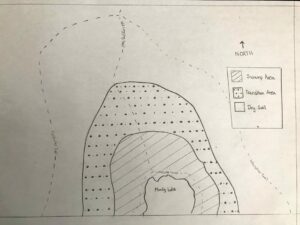
For my sampling strategy I opted for haphazard sampling of individual rose plants. For the initial data collection in Module 3 I selected one plant in each of the following height ranges: 1-50cm, 51-100cm, 101-150cm, 151-200cm, and above 201cm. The reason why I have opted for haphazard sampling over random or systematic is that the area where the roses are located is specific and not large. Dividing the land into quadrats would also be exceedingly difficult due to the thickness of the roses and surrounding underbrush.  There are many unbranched wild rose plants that fall within each of the height ranges outlined above. Therefore it was easy to find one from each height range to observe for the initial data collection. The only difficulties in sample collection are the thickness of the underbrush making it tough to access the roses, and that the vegetative buds are beginning to form into leaves and small branches.

The initial data was not overly surprising. The sample size was much to small to derive any meaningful conclusions, however, the initial data supported my theory that the spacing of the vegetative buds is not related to the height of the plant. I also collected data on the number of vegetative buds on each individual plant and the distance from the apical bud to the lowest vegetative bud. These additional pieces of information did not provide any interesting information and I do not believe that I will continue to collect these data as I move forward with this experiment.

I plan to continue to use the same sampling method in an equal number of individual plants will be observed in each height range. I believe that by simply haphazardly observing many more individual plants in each height range I will be able to have enough measurements to perform an ANNOVA analysis.

Blog post 3: Ongoing Field Observations

User:  | Open Learning Faculty Member: 


May 13 5:55 pm

Weather: 18 degrees, mostly sunny

I have chosen to study the factors that affect sword fern (Polystichum munitum) growth. From my previous trip, I noticed that sword ferns are densely populated in the middle of the forest and grow sporadically away from the center. This difference in fern density leads me to believe that there are conditions that favor fern growth in the center of the forest as opposed to the outskirts of the forest.

I have chosen 3 different areas to study. Each having similar composition in topsoil but differ in elevation and position.

The first area is close to the northern entrance of the forest at about 20 m elevation. It is heavily shaded by trees and only one fern is seen growing on a mound next to a covered manhole. I have counted 8 fronds on this fern, each of which grows at about less than 2 feet. The surface of this soil seems dry and is covered heavily by sticks, pebbles, and smaller unidentifiable plants growing around the fern.

The second area is at 25 m elevation moving west. This area is the closest to the center of the forest where there is a higher population of sword ferns growing closer together with longer fronds (approximately 4 feet). The area is moderately shaded with few spots where sunlight can peak through. Many of the ferns in this area appear to have spores. The fronds here are fuzzy in appearance and curl inwards at the tips. Soil in this area is composed of mostly sticks and pebbles, though in comparison to the first and third area, the soil looks darker.

The third area is at 30 m elevation. Here, there are only 3 ferns growing about 6 feet away from each other and there is little shade. Frond length is similar to the first area at about 2 feet or less in length with some fronds looking wilted/drooping. The soil here is mostly covered by sticks and there is little vegetation surrounding the ferns.

Patterns I have observed from this trip are that ferns found toward the center of the forest look much healthier and their fronds grow larger in comparison to ferns grown away from the center, which are smaller and have a larger portion of wilting/drooping fronds. Most of the ferns I had observed in all 3 areas grew on a slope or a mound. The soil in the center of the forest is also much darker looking than the other two areas. I am particularly interested in this difference as I suspect the difference in soil properties plays a role in fern growth. In addition to the varying soil properties, I believe slope and light variability also affect how favorable fern growth will be. However, I would like to focus my studies on how soil moisture and pH affects the length at which fronds grow as I believe it would be the easiest factor to study. I hypothesize that the availability of soil moisture will have an effect on the frond length of sword ferns (Polystichum munitum). I predict that as the level of moisture in soil increases, frond length will also increase.

My response variable will be the length at which fern fronds grow and my predictor variable will be the level of soil moisture. The response variable would be continuous, and the predictor variable would be categorical.

Post 3: Ongoing Field Observations

User:  | Open Learning Faculty Member: 


Date: 18 May 2021
Weather: Mostly Cloudy, no wind, no precipitation
Temperature: 12°C

I returned to my field study site and made my way to Mundy Lake. Mundy Park has lots of western Sword Ferns throughout the park yet near the lake there were very few. As I made my way away from the lake, I noticed the soil became drier and the number of Sword Ferns slowly increased. This environmental gradient sparked my curiosity and I decided that this area would be my location for my field study. I used Google Maps on my cellphone to mark GPS coordinates in order to map out this environmental gradient.

1. Identify the organism or biological attribute that you plan to study.

Western Sword Ferns.

2. Use your field journal to document observations of your organism or biological attribute along an environmental gradient. Choose at least three locations along the gradient and observe and record any changes in the distribution, abundance, or character of your object of study.

EnvironmentalGradient
Environmental Gradient

Near Mundy lake it is marshy, and the soil is consistently wet. This area had very few Western Sword Ferns. As I moved away from the lake the elevation increases slightly and the soil becomes more dry and solid. Along this gradient, the number of western sword ferns increased with increased distance from the lake. The greatest number of sword ferns were found in the dry soil and the lowest amount was found in the swamp area.

3. Think about underlying processes that may cause any patterns that you have observed. Postulate one hypothesis and make one formal prediction based on that hypothesis. Your hypothesis may include the environmental gradient; however, if you come up with a hypothesis that you want to pursue within one part of the gradient or one site, that is acceptable as well.

Process

The underlining process that may be behind this pattern is the amount of water in the soil. The soil I observed across this gradient included dry, muddy, as well as standing water.

Since sword ferns are preferentially located farther away from the lake, I hypothesize that soil moisture is a determining factor in the concentration of sword ferns in this area of Mundy Park.

 Hypothesis

Sword Fern density is greater in soil that relatively dry and solid rather than saturated mushy soil or standing water.

Predictions

Sword Ferns are more likely to develop in areas wherein areas that are not marshy.

Sword Ferns are more likely to develop farther away from the lake.

Sword Ferns are more likely to develop in nutrient-rich soil.

4. Based on your hypothesis and prediction, list one potential response variable and one potential explanatory variable and whether they would be categorical or continuous. Use the experimental design tutorial to help you with this.

Potential response variable: occurrence of Sword Ferns (Categorical).

Potential explanatory variable: Soil moisture defined as solid, spongy, standing water (Categorical).

This study would be tabular since both variables are categorical.

Blog post 2: Sources of Scientific Information

User:  | Open Learning Faculty Member: 


The source I found was an eBook from the online library through TRU. The book is called “Source of Birds of British Columbia: A Photographic Journey” by Glenn Bartley. This source will be useful while I am trying to determine bird species at the Esquimalt Lagoon. This source is considered as non-academic material because it does not follow the criteria of having a bibliography or in-text citations.

Link to the eBook https://ezproxy.tru.ca/login?url=https://search.ebscohost.com/login.aspx?direct=true&db=nlebk&AN=561136&site=eds-live&scope=site&ebv=EB&ppid=pp_53

Post 1: Observations

User:  | Open Learning Faculty Member: 


I have selected an area of Esquimalt Lagoon located in Victoria on Vancouver Island, B.C. The area of interest is beside the ocean and in a little nook with a wetlands area some rocky shoreline and a grassy patch that is close to the road. There is fresh water run off from a drain that leads to the ocean shore. There is abundance of plant species including Oregon Grape and lots of tall grasses. The location was visited at noon on a sunny spring day in May and is approximately 50 ft by 40 ft. The spot I am interested in is full of birds of various species which makes sense since the lagoon is considered a bird sanctuary and I believe the birds would be great potential subjects. Three questions that could be formed are; What are the different bird species found to be eating and why?, Which is the proportion of strictly migrant birds vs strictly native ones in the area and suppose why?, Which birds more frequently stay in the area at different times of the day and suppose why?

Blog Post 4: Sampling Strategies

User:  | Open Learning Faculty Member: 


Create a blog post describing the results of the three sampling strategies you used in the virtual forest tutorial. Which technique had the fastest estimated sampling time?

Systematic sampling was found to be faster than random or haphazard sampling. Systematic sampling took 12 hours and 35 minutes, random sampling took 13 hours and 50 minutes, and haphazard sampling took 12 hours and 54 minutes.

Compare the percentage error of the different strategies for the two most common and two rarest species.

Systematic Sampling:

Two Most Common Species:

Eastern Hemlock density actual was 469.9 versus 388.0 calculated is a 17.4% difference.

Sweet Birch density actual was 117.5 versus 148.0 calculated is a 20.6% difference.

Two Rarest Species:

Striped Maple density actual was 17.5 versus 40.0 calculated is a 56.2% difference.

White Pine density actual was 8.4 versus 20.0 calculated is a 58% difference.

Random Sampling:

Two Most Common Species:

Eastern Hemlock density actual was 469.9 versus 496.2 calculated is a 5.3% difference.

Sweet Birch density actual was 117.5 versus 107.7 calculated is an 8.3% difference.

To Rarest Species:

Striped Maple density actual was 17.5 versus 7.7 calculated is a 56% difference.

White Pine density actual was 8.4 versus 3.8 calculated is a 54.8% difference.

Haphazard Sampling:

Two Most Common Species:

Eastern Hemlock density actual was 469.9 versus 484.0 calculated is a 2.9% difference.

Sweet Birch density actual was 117.5 versus 140.0 calculated is a 16.1% difference.

Two Rarest Species:

Striped Maple density actual was 17.5 versus 32.0 calculated is a 41.7% difference.

White Pine density actual was 8.4 versus 8.0 calculated is a 4.8% difference.

Did the accuracy change with species abundance?

Both systematic and random sampling had greater accuracy with species abundance. However, haphazard sampling resulted in both the most common and rarest species having greater accuracy.

Was one sampling strategy more accurate than another?

Random sampling can be more accurate than systematic due to periodic ordering. However, haphazard had greater accuracy, which may be due to increased homogenous communities, leading to a greater community representation.

Blog Post 4 – Sampling Strategies

User:  | Open Learning Faculty Member: 


For the tree sampling program, the three different sampling methodologies chosen were area-based random, systematic, and haphazard sampling. The most efficient methodology was random sampling, which was 20 minutes faster to complete compared to haphazard sampling (12 hours 8 minutes versus 12 hours 28 minutes). Systematic sampling was the most accurate for estimating diversity, with a Shannon-Wiener diversity index value of 1.5, which is the same at the true value. Random sampling was the least accurate, with a value of 1.3

The two most common tree species in the study area are eastern hemlock and sweet birch. Systematic sampling was the most accurate in estimating density of eastern hemlock, with a percentage error of 11.5% compared to random (18.4%), and haphazard (21.5%). Random sampling was the most accurate in estimating density of sweet birch, with a percentage error of 0.08% compared to haphazard (6.4%) and systematic (21.7%).

The two most rare species in the study area are striped maple and white pine. Both random and systematic sampling methodologies failed to record this species, while haphazard was fairly accurate in estimating density with a percentage error of 4.6%. All methodologies were poor at estimating density of white pine. Systematic was the most accurate with a percentage error of 90.5%, while haphazard had a percentage error of 247.6%. Random sampling failed to record this species.

The accuracy of density estimates declined the more rare the tree species were. Twenty-four sample points were likely not a sufficient number as multiple methodologies had large discrepancies between estimated and actual densities of multiple species, while some methodologies failed to record some species at all.

Blog Post 9: Field Research Reflections.

User:  | Open Learning Faculty Member: 


Doing a field research was a great experience for me, not only as a student fascinated by Biological processes, but also as an individual who did not always pay much attention to the ecosystems around her. Some words that I could use to describe the overall experience include eye opening, intellectually challenging, and inquisitive.

During the process of designing the field experiment, I decided to use the systemic sampling strategy to help me avoid experimenter bias while choosing the samples. Initially, I thought I could randomly select the first bean plant, and then systemically select the next samples. However, later in the experiment I realised that the garden beds were not large enough for the samples to be spread out perfectly in fives (the random number generated using excel). Thus, I decided to use the same approach, but this time recording every third plant instead of the fifth.

Another change that I made while implementing the experiment was that I only collected data from 2 garden beds (locations) instead of 3, which were from the original plan. This was due to the inaccessibility of the garden bed because of the long fence around it, unfortunately I could not reach individual beans without making damage.

Finally, I can confidently say that engaging in the practice of ecology increased my appreciation for how ecological theory is developed. I learned that it starts as a simple process from observation, which grows over time as the experimenter finds certain patterns and organizations that sometimes represents significant processes in the surrounding communities, and even ecosystems.

Blog Post 3 – Ongoing Dufferin Wetlands Observations

User:  | Open Learning Faculty Member: 


I returned to the Dufferin Park Wetlands on May 13, 2021 at approximately 16:40 hours, and decided to sketch a map (attached) to assist with further observations. I must note that the majority of the vegetation in this area is still in the process of recovering from the winter season.

On my way over to the wetlands, I noticed a “trough” that paralleled the sidewalk and tennis courts which featured some of the same vegetation that had I originally noted in my first blog post. I also made note of the two circular canal areas near the information/shade hut as they featured many similarities in vegetation to the wetlands, but to a greater degree than the “trough” noted earlier. Furthermore, during my observations, I noticed that only one bird attended the “trough” area and that two species of birds attended the circular canals.

These observations lead me to thinking that the diversity in wetland vegetation between these sites may have an affect on the diversity of bird species that interact with them. In short, I was lead to the following hypothesis and prediction:

  • A greater degree of biodiversity in wetland vegetation will lead to a greater degree of biodiversity in bird species that will interact with the vegetation.
  • I predict that more birds will attend areas that have more biodiverse vegetation more often than areas with less biodiversity.

The predictor variable in this case would be the number of plant species in a given area, and the response variable would be the number of birds that interact with the vegetation. I believe that the predictor variable will be continuous, but this may change as the vegetation develops over the spring and summer seasons. As such, this variable may change marginally (which remains to be seen) and may in fact become a categorical variable in time. The response variable in this case is categorical, so I believe that this will be either a logistic regression or tabular experiment.

I plan to use sections of the main wetlands area, the circular canals, and “trough” as there is a clear gradient in the biodiversity of plants between these areas.

Blog Post #4 – Virtual Forests Exercise

User:  | Open Learning Faculty Member: 


Of the systematic, random, and haphazard sampling techniques used, I noted that each method presents its own advantages and disadvantages. For example, the systematic sampling strategy appeared to be the most straight-forward and least time-consuming method, but only focused on a centralized area of the landscape. The random and haphazard methods presented as very similar (especially because I opted to use no bias in my haphazard site selections) and appeared to be more complex, labour-intensive, and time consuming than the systematic method. However, these methods appeared to give a more complete picture of the landscape as the samples were not limited by any criteria, save for chance (which can unfortunately not work in our favour at the best of times, it seems).

I was under the impression that the sampling times would greatly vary, but was surprised to find that the estimations generated by the virtual program were marginally different. The sampling methods clocked in at the following times:

  • Systematic: 12 hours, 36 minutes
  • Random: 12 hours, 53 minutes
  • Haphazard: 12 hours, 37 minutes

I was unsurprised to find that the systematic method was estimated to be the fastest, but was even more surprised to find how close the haphazard method measured in. Regardless, I feel that the random and haphazard sampling methods could be highly variable due to the randomness of how sites are selected.

When examining accuracy, I had assumed that the random sampling method would be best, which, judging by the data comparisons appeared to have been somewhat correct.

The percentage error for the two most common tree species measured as:

  • Eastern Hemlock
    • Systematic: 17.4% error
    • Random: 19.7% error
    • Haphazard: 16.1% error
  • Sweet Birch
    • Systematic: 38.7% error
    • Random: 18.5% error
    • Haphazard: 41.9% error

The percentage error of the least common tree species measured as:

  • Striped Maple
    • Systematic: 60.0% error
    • Random: 4.6% error
    • Haphazard: 4.6% error
  • White Pine
    • Systematic: 100% error
    • Random: 100% error
    • Haphazard: 1.2% error

Overall, the random method appeared to be the most accurate sampling method for measuring the most abundant species, while the haphazard method appeared to be the most accurate when measuring the least abundant species. With all things considered, the random and haphazard sampling methods appear to be the most accurate and holistic methods to use, even though they are more time consuming than the systematic method.