Recent Posts

Blog Post #6 – Data Collection

User:  | Open Learning Faculty Member: 


For my initial data collection, I only looked at three trees, systematically sampled on the North side of the park, as a whole, but as my observations went on, I decided to look at each tree in five different sections from top to bottom. For each of these sections, I noted down that percentage of leave that haven’t changed color yet, and then once I have all five sections, I took the average percentage of the total leaves that haven’t changed color. Each observation was initially taken three days apart, but after some revision, I decided it would be best to take observations every one or two days as the humidity level and leaf color changes more that I anticipated. This way, I could potentially get more accurate results.

I didn’t have too much trouble implementing my design, but there definitely had to be some changes like taking observations for frequently and using a hygrometer to better measure the humidity level.

So far, my observations do support my hypothesis that when humidity level decreases, than the leaf color change increases. But there are some observations that don’t follow exactly.

Blog Post 4: Sampling Strategies

User:  | Open Learning Faculty Member: 


Which technique had the fastest estimated sampling time?: Haphazard was the fastest.

Compare the percentage error of the different strategies for the two most common and two rarest species.: both were right skewed, however haphazard sampling resulted in less error dispersion, where as random sampling showed a clearer dispersion of error. Seen as how they both skew in roughly the same way, I would conclude that random sampling is accurately representing possible error, where as haphazard may be showing a tendency to show false positive.

Further thoughts: It may also be that with a right hand skew, plus less diffuse error distribution in the haphazard model may actually be a fat tail. If this is the case, then some very important outliers could be hiding in that tail. On second thought, I don’t think I’d want to use this sampling technique where missing the effects of outlying, or phenomenon could have a major impact on stake holders involved in decision making. I wouldn’t use this in helping with ecological assessments around environmental safety, conservation issues regarding extremely endangered species, or economically and culturally vital species, such as salmon or herring populations. If there is error, the randomized model seems represents it more effectively, with a more dispersed deviation around the mean, there by prevent the right skew kurtosis.

Did the accuracy change with species abundance?: No, it didn’t seem to. Although, this may reflect the fact that when I sampled in haphazard sampling, I followed a pattern, and did not attempt to emulate a random pattern. I may have to try sampling again.

Was one sampling strategy more accurate than another? I believe so. I think random sampling shows a more accurate distribution of the deviation. However, haphazard is faster, and easier. If the errors in haphazard are predictable, and can accounted for, it may still be appropriate under certain circumstances.

Blog Post 3: Ongoing Field Observations

User:  | Open Learning Faculty Member: 


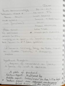
My third blog post comes with a bit of a delay, fortunate I did take notes on the last day of observations, as well as taking photographs of the evidence of the bog fire from last year.

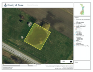
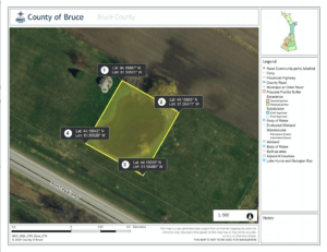
Before proceeding, I’d like to direct the reader’s attention to an article from last year that reported on this fire, and it’s location. I would like to do this in order to provide verification of the bog fire, the time and location at which occured.

Year in review: Bog fire burned: Richmond’s wildfire was one of the biggest blazes in local history.

From the article:

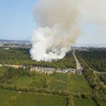
“The summer of 2018 was one of the hottest ever recorded in B.C. and Friday, July 27 is a day that will live long in the memory of Richmond’s fire department.

Early morning reports of smoke coming out of the peat woodland at the DND Lands, near Westminster Highway and Shell Road, quickly developed into a wildfire.” (Campbell, 2018).

I’ve also been trying to determine how to demonstrate to the readers, here, that the burnt over areas I plan on sampling in did indeed experience that same fire a year ago. It occurred to me that in response to their canopies being destroyed by the fire, many of the invasive blueberry, Vaccinium corymbosum, would probably have begun to re-sprout this year. The new vegetative growth, if it was only from this years growth, should not have had time to lignify, so if I observe an abundance of such growth (all green, with no lignified, woody tissues present) then this should be a demonstrable indicator of a fire having occurred within the area of observation in the season prior(summer 2018) to this year’s growing season (2019).

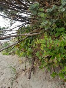
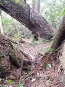
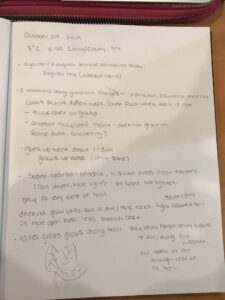
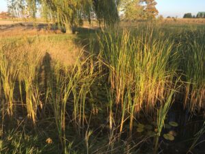
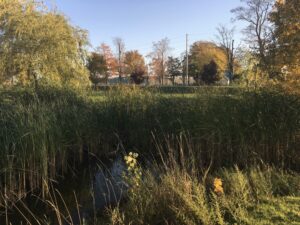
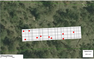
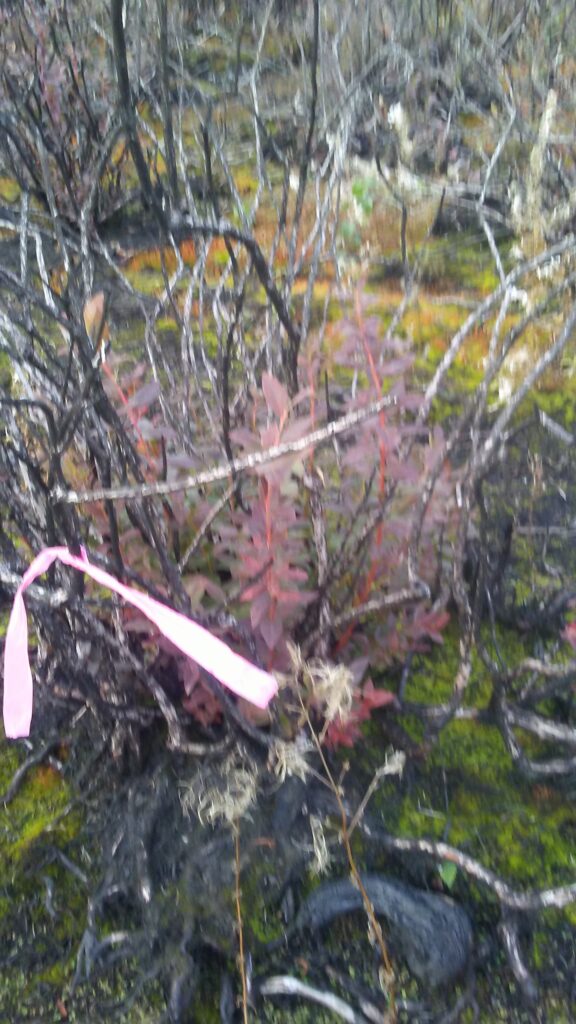
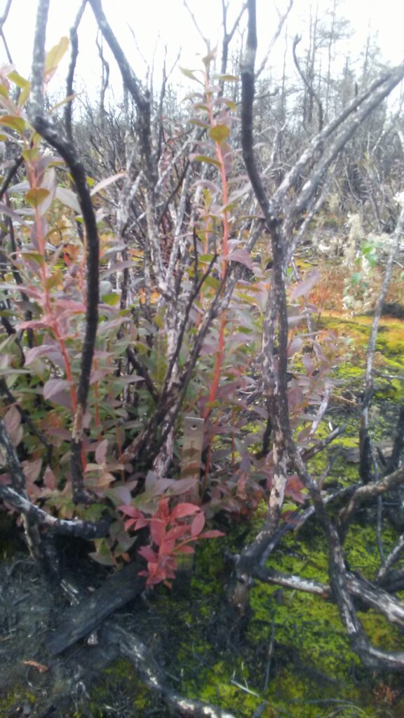
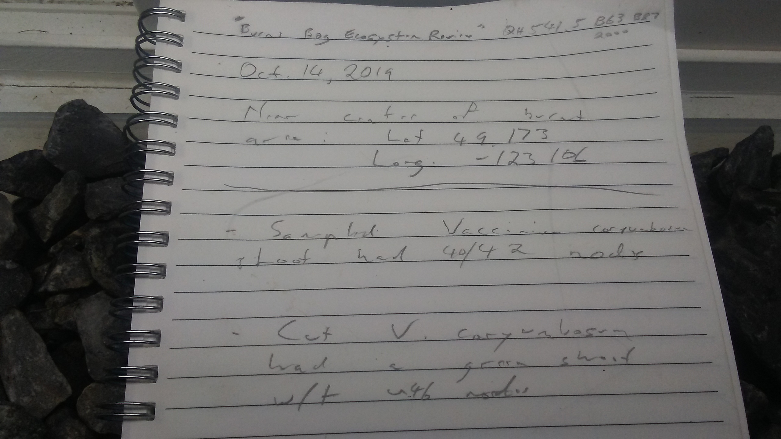
So I returned to the bog at the DND Lands on October 14th, 2019, and made some observations. According to the time stamp in my photos, the time was 5:35pm. Through out the areas that still had residual suit and char, many V. corymbosum plants, who’s canopies had been destroyed, but who’s crowns had not been damaged, showed obvious signs of vigorous greens growth, little to none of which had lignified, or only had very little newly lignified tissue at the bases of the new stems. I also took photographs of this growth, to show that there could only have been a single season’s growth since the last fire, and that fire must have occurred in the areas I will be making my observations.

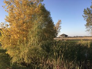
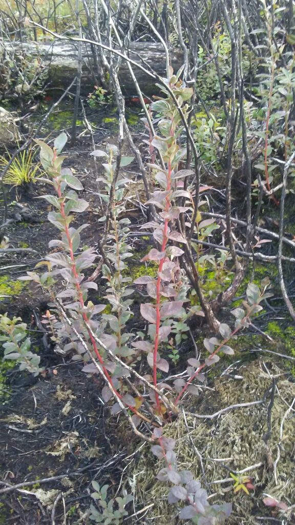
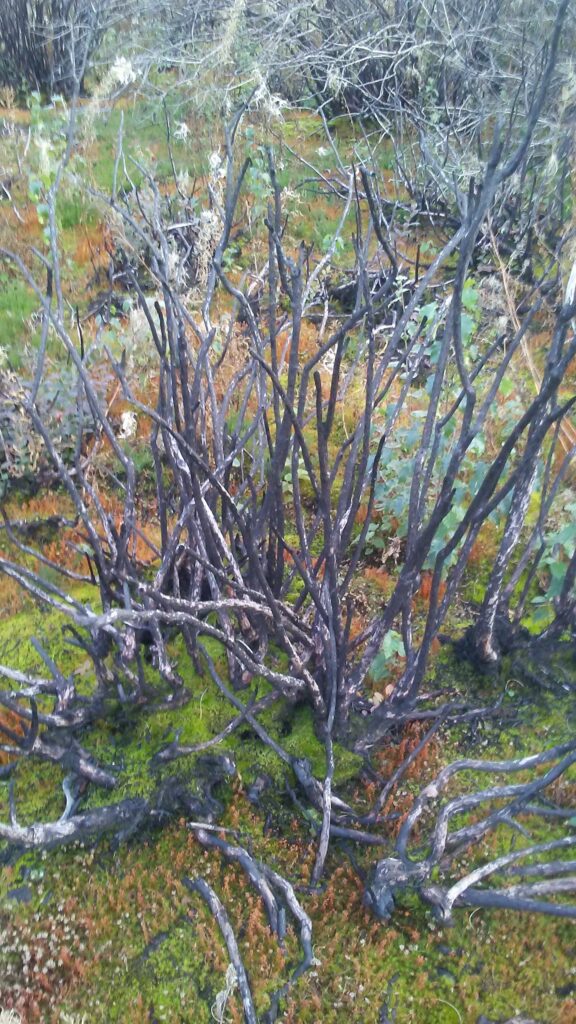
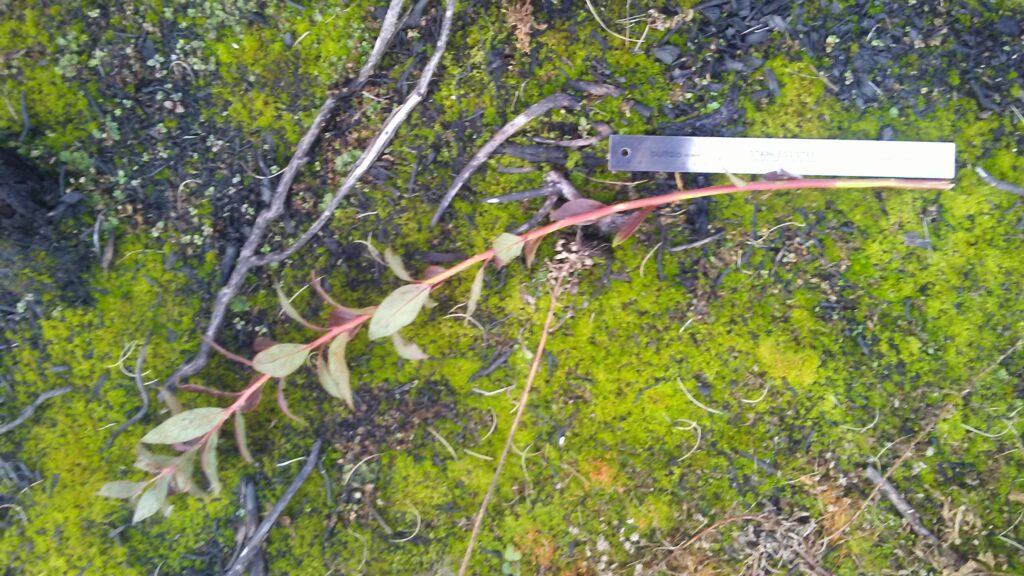
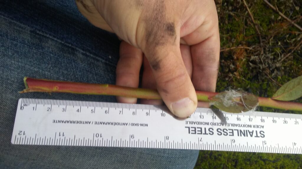
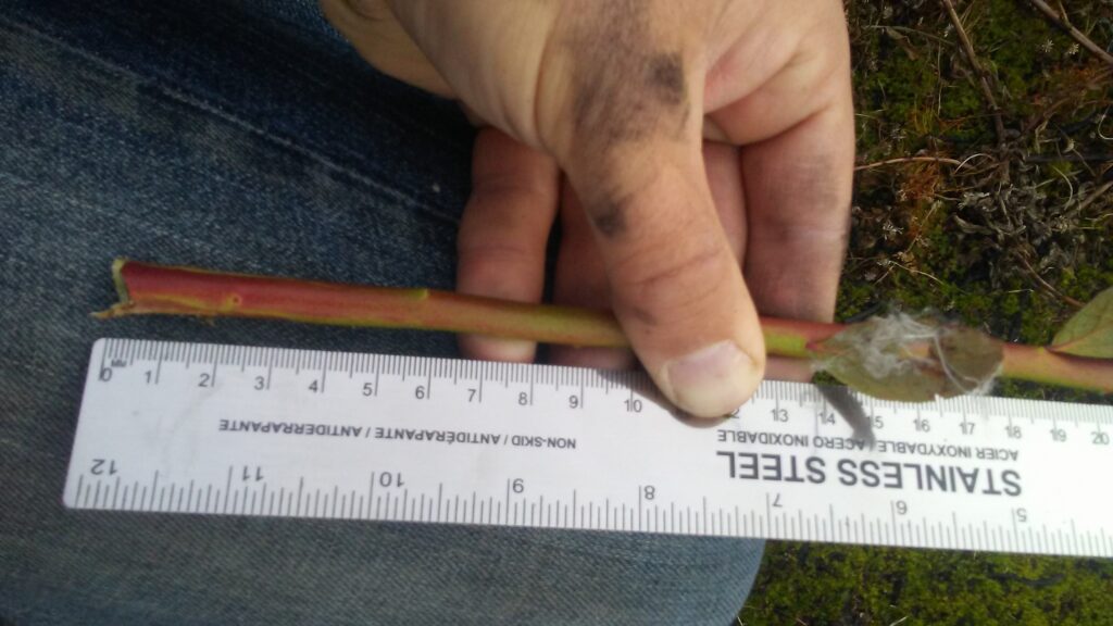
In the fifth picture I photographed the branch to be sampled while still attached to the original plant. According to my notes, the branch sampled had 42 nodes. If you can see the foot long ruler under the burnt blueberry bush, you’ll see that the branch is about three times longer than the ruler, so the branch had grown roughly a meter in one growing season. This may seem like a lot of growth, but many species of plants exhibit this response to having their canopy’s destroyed, especially ericacasious plants. In both the fifth, sixth, and seventh photos, we can see that the entire branch is composed of new, green tissues, and has virtually no lignified materials. Given the reports of fire in this area from last year (2018), the obvious evidence of recent fires in the immediate area (black suit, blackened peat, chard woody material, clearly visibly in all the photos) and the evidence of a single season’s worth of growth in the V. corymbosum plants, we can conclude with relative confidence that there was a bog fire in the summer of 2018 within the DND Lands, and, more importantly,  in the areas where I will be observing plant fire responses.


Blog Post Three: Ongoing Observations by E. C. Bell

User:  | Open Learning Faculty Member: 


Blog Post Three: Ongoing Observations by E. C. Bell

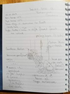
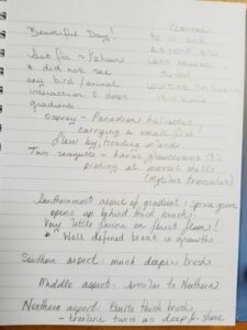
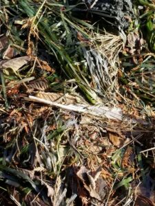
Feather embedded in seaweed, grasses & leaves at Inlet site.

The biological attribute of interest of my study stems from the comparison of two gradients approximately 5km apart which have differences in physical traits of the transitions from forest to shoreline affected by environmental factors, including weather patterns and soil structure. The two gradients lie across Esowista Peninsula from each other, the Eastern inlet site and the Western coastal site. The ‘piece’ in this comparison will be the variance in ecotone transition and the ‘pattern’ will be the similarities in species with distinct differences in their physical traits and interactions. The elevation of the inlet location has a more gradual slope directly through the shifts in environmental factors. There are pebbles that increase in size to boulders of beach-ball size at the forest line, more of both seaweeds than grasses towards the pebbles, holding feathers, shells and bits of driftwood. The coastal site rises steeply for approximately 1m from sand to brush, covered in grasses, some seaweeds, yet then tapers off to a gradual slope covered in thick brush, mostly Gaultheria shallon. There is a fairly distinct line where stunted Pinus contorta takes over, looking very bonsai in shape of the needles with a sparse undergrowth – very little fauna of any species was growing on the forest floor. It was a messy situation getting through the thick brush.

Western Coastal site                      Eastern Inlet site behind the shoreline brush

The hypothesis I am considering for this comparison of two environmental gradients is: there will be degrees of variation in the expression of populations and their densities within existing species due to tidal patterns and differences in weather exposure experienced over time. The ensuing prediction is: because of the different micro climates created by topographical land mass and Eastern facing aspect, the inlet site will have more biological diversity but less density in flora and interacting fauna than the Western facing aspect due to the open ocean exposure and pattern of winter storms, which have both shaped the gradients and variance that there exist. One categorical response variable may be variance in the dimensions of leaf size in Gaultheria shallon assuming that each location receives a similar exposure to sunlight. One continuous explanatory variable may be exposure to wind over a range of temperatures.


E. Carmen Bell

Blog Post 3: Ongoing Field Observations

User:  | Open Learning Faculty Member: 


The organism I plan on observing is English ivy (Hedera helix)

Since observing this vine-like plant last time I visited my study site, I researched the name of it and see that it is an invasive species in southwestern B.C.

When observing my study site, there is not a gradient of elevation, but there is a gradient of sunlight. There is a densely forested area that has lots of branch cover and little sunlight. Here the Ivy grows thick and covers stumps, fallen trees and the ground where the trail is not. Moving closer to the beginning of the trailhead, there is less branch cover and the ground is slightly drier. There are small patches of the Ivy, but the leaves are much smaller, and they grow in groups. Along the length of the open trail, there is no trail cover and the ground is much drier. Long grasses grow here, and there was no sign of the Ivy. It appears that sunlight is the underlying process for where the Ivy grows. Perhaps the plant is not so picky about where it grows/what species it is growing around but is more dependant on sunlight. This leads me to hypothesize that the English Ivy grows in shaded, damper areas.

The response variable here could potentially be the abundance of English Ivy growing (continuous) and the explanatory variable could be access to sunlight (categorical).


Post 4. Sampling Strategies

User:  | Open Learning Faculty Member: 


Systematic sampling had the fastest estimated sampling time (12 hours, 37 minutes). Table 1 below summarizes the percent error and estimated total sampling time for each sampling method (systematic, random, haphazard), two most abundant (Eastern Hemlock and Sweet Birch) and two most rare (Striped Maple and White Pine) tree species.

Percent error was higher for the two most rare tree species (Table 1). Random and systematic sampling methods had similar accuracies, and both provided more accurate results than the haphazard sampling method (Table 1).

Table 1. Frequency of the two most rare and most abundant tree species in the field sampling tutorial.

Sampling Method Systematic Random Haphazard
Tree Species Estimated Frequency (%) True Frequency (%) % Error Estimated Frequency (%) True Frequency (%) % Error Estimated Frequency (%) True Frequency (%) % Error
Eastern Hemlock (1) 76 73 4 65 73 11 80 73 10
Sweet Birch (1) 48 43 12 46 43 7 44 43 2
Striped Maple (2) 0 6 100 12 6 100 20 6 233
White Pine (2) 4 4 0 4 4 0 8 4 100
Total Time (hours.minutes) 12.37 13.43 13.2
1 = Most common tree species
2 = Most rare tree species
Note: % Error calculated as an absolute value
% E = (Estimated-True/True)*100


Blog Post #5 – Design Reflections

User:  | Open Learning Faculty Member: 


At first I wasn’t sure how I would measure the change in leaf colour with changes in humidity levels, but I think measuring the percentage of changed leaves this way is going okay. I couldn’t think of another efficient way of collecting this data. After four observations and noting down the humidity levels each day of observation, I may need to do more, perhaps every day or two, instead of three days like what I’m doing currently. This way, I may be able to see changes more steadily than a big change. I’m also going to bring out a humidity detector to more accurately measure the humidity in the park at that time.

I am surprised to see though, that leaves at the top of the tree changed much faster than those closer to the bottom. As well as seeing that leaves further on the outside of the branches change faster than the inner parts of the branches, where it is also more dense.

I’m not sure if I’ll keep how the data is shown in a table, but there is a way to better sum up all the information with a different visual.

Blog Post 6: Data Collection

User:  | Open Learning Faculty Member: 


During my initial observations I determined the size of my entire study area (Figure 1 and 2). The size of is approximately 28m by 30m, which I then divided into four quadrants 14m by 15m. As discussed in my previous post after trial and error it was determined individually counting the species to research diversity and population density of invasive pond weeds would be best represented in a range. By utilizing a chart, I have visited the pond a handful of times, once a week and made note of the population densities for various plant species, based on their location surrounding the pond (N,E,W,S) and the ratio of interacting factors.


Figure 1: Study Area


Figure 2: Study Area Coordinates

The following photos were taken October 20, 2019 at 5:00 pm on a sunny fall evening. The weather was approximately 10 degrees celsius and somewhat windy.

Blog Post 5: Design Reflections

User:  | Open Learning Faculty Member: 


Although my data collection may be more straightforward then other studies that involve in depth measurements and larger study areas, I still found I had some difficulty solidifying my study areas. Due to the fact the pond I am studying is irregularity shaped it was difficult to create study areas that were the exact same area and consistent with one another (i.e. similar amount of grassed area, pond water depth, etc). I used air photos and online mapping tools to create a rectangle surrounding the pond and then divided the rectangle evenly in four. The quadrants were divided by direction which was one pro as that is consistent, NW, NE, SE, SW and will be utilized as a variable. I found it difficult to conduct accurate population density of the species by counting for the heavily populated species since it was difficulty to differentiate between individuals and keep track, to counteract this I decided to create a range rather than an exact number. This may be subjective and difficult to confirm accuracy, so I repeated this population count once a week for 8 weeks. There was little to no variation between each visit, especially with mature vegetation like trees. However, I also believe this information is bias to the current season being fall compared to obviously Winter, Spring and Summer. I am confident supplementary research will assist me in supporting my data and I look forward to research pond management and diversity further.

Blog Post 5: Design Reflections

User:  | Open Learning Faculty Member: 


During my initial data collection, summarised in my Small Assignment 1 there were a few difficulties in implementing my sampling strategy. I was using 1.5 m by 1.5 m quadrats (2.25 m2) as my sampling unit along a transect, which in the field I measured out and delineated with tent pegs at each location (see Figure 1 below). I found this to be inefficient and time consuming. I also calculated the percentage slope by using tent pegs and measuring rise over run (over a 1 m distance), again I found myself measuring 1 m out at every quadrat, which again was time consuming.

Figure 1. Illustrating an east-west transect, with 1.5 m by 1.5 m quadrats (2.25 m2) spaced 5 m apart, alternating north and south of the transect.

The data was somewhat surprising, in all five replicates there was no common snowberry present which I didn’t expect. I also found the percentage slope I calculated at each quadrat was steeper in the Upland Area than I had visually assumed. I am curious to calculate the slope in my other areas (Transition Area and Riparian Area) to assess the difference in percentage slope between the three sites, they may be different to what I had expected from my visual assessment. I would also like the percentage slope between my three sites to be different from one another, to represent a flat, moderate and steep slope. Once I calculate the slope percentage in each three sites, the results may shift my prediction. I am currently predicting snowberry to be present on slopes less than 20% grade, which may change to slopes less than 30% grade, or on slopes less than 10% grade (depending on the results of my field sampling program).

I plan to modify my sampling technique in the field by improving my equipment. I plan to make a 1.5 m by 1.5 m PVC quadrat which will have markers every 0.5 m. Having the PVC quadrat will save time at each location and creating a marker every 0.5 m will improve efficiency when I am calculating slope at a 1 m horizontal distance.

My sampling technique will also be modified by increasing my replicates to 10 quadrats per site as a minimum. I may also change my sampling technique from a transect to simple random as I want to increase the independence from one quadrat to the next. To do this, I will create a map showing each site represented by a 10 m by 50 m polygon: Riparian Area, Transition Area and Upland Area. Based on the polygon I will create an x and y axis and use a random number generator to locate the 10 quadrats within each site (see Figure 2 below for 10 quadrats within the Upland Area). I will use the map and the numbers generated to find the sampling locations in the field. This technique in the field may take more time to locate each quadrat, however this modified technique will increase my independence between quadrat as it’s a larger sample size (10 m by 50 m) compared to the transect method (3 m by 27.5 m) and this technique will help to prevent bias in the field.

Figure 2. Illustrating an alternative random sampling technique where 10 replicates are randomly located within a 10 m by 50 m polygon representing the Upland Area.

I will be improving the efficiency of my sampling protocol by using a standard 1.5 m by 1.5 m PVC quadrat, however I will potentially be increasing my time in the field because of the time required to locate each sample. I think my modifications will improve the independence, avoid bias and decrease the percentage error.