Recent Posts

Blog Post #4 – Sampling Strategies

User:  | Open Learning Faculty Member: 


For sampling simulation of Snyder-Middleswarth Site using area-based sampling.

The fastest estimated sampling time was haphazard sampling at 12 hours and 27 minutes, 11 minutes faster than random and 9 minutes faster than systematic sampling.

Eastern Hemlock (common): haphazard – 2.9% ; random – 26.4% ; systematic – 12.3%

Red Maple (common): haphazard – 8.7% ; random – 12.1% ; systematic – 12.5%

Striped Maple (rare): haphazard – 65.7% ; random – 138.3% ; systematic – 8.6%

White Pine (rare); haphazard – 50.0% ; random – 100% ; systematic – 100%

Most accurate sampling strategy for common species (Eastern Hemlock and Red Maple) is haphazard sampling, and the most accurate for rare species (Striped Maple and White Pine) is also haphazard sampling. In this case, haphazard sampling was more accurate compared to random and systematic.

Accuracy, in general, was better with species that are more common, and worse with species that are more rare. The accuracy decreased for rare species as all percentage errors for each of the three sampling techniques increased.

24 sampling points is not a sufficient number of sampling points. With the abundance of each species varying greatly throughout the study area, only having 24 points doesn’t properly represent the number of species. There are a lot of missed species.


Blog #1 Observations by E. Carmen Bell

User:  | Open Learning Faculty Member: 


Biology 3021
Community and Ecosystem Ecology
Blogs by E. Carmen Bell
Blog Post 1: Observations
Already, this Ecological Field Study has taught me many things. It has taken me weeks to settle
on potential field study locations and considerations. I believe this has to do with my perspective being
originally too narrow for the assignment. I was searching for a particularly interesting angle from
which I could make a detailed study and inventory and may have been attempting a prescibed outcome.
However, I now understand that my scope needed to open to a wider lens. Time spent in two situations,
as well as, revisiting the Biology 3021 requirements, guided me to observe the patterns of interacting
species of flora and fauna.
Comparing two potential field plot locations, situated across the Esowista Peninsula from each
other, may provide an interesting exploration into the similarities and differences between coastal
shorelines on the inside and the outside of the peninsula. The inlet plot location is slightly NE from the
Ecolodge on the satellite image below. The outside coastal plot is towards the bottom of the image,
along Chesterman Beach and before the spit that looks like the tail of a ‘Y’.


Credit to Google Maps

Salt water tidal fluctuations make contact with the inlet plot location at high tides when close in time to
the new and full moons. Both sites are close to high tide levels, the Eastern site is less than 5 meters and the Western site is approximately 20 meters to high tide water lines at this time of year. Both sites surely receive wave action during storm surges. During today’s observations, it was a flooding tide, less full by one to two hours.
Picea sitchensis, Thuja plicata and Tsuga heterophylla trees were interwoven with Gaultheria shallon
and Vaccinium parvifolium, whom still had the odd berry dangling. There were Blechnum spicant and
Polystichum munitum ferns and grasses of which I have yet to identify. I observed patterns of layered
growth on nurse logs and transitioning ecotones over depths of 5 meters from where the forest becomes
the beach. While on location at the sites, I have observed an eagle, osprey, heron, robin, blue jay and
today, a delightful small bird with a yellow patch that I must identify. Different times of day may
provide for different observations of bird life.


East side of Esowista Peninsula     West side of Esowista Peninsula

My visits to these locations have been at high tide and low tide, morning and late afternoon.
They are each approximately ten meters wide and 5 meters deep from the shoreline into the forest. The
gradients have a similar topographical slope upwards into the bush. Today, 3-10-2019, I was at the inlet
location at 1500 hours and the sandy beach location on the outside of the penninsula at 1700 hours.
There was a light wind of about 10 km/hr, the temperature was 13 degrees Celsius, there were cumulus
clouds in a patchy sky that gave pockets of gentle sunshine. No fog was visible at these times. The inlet
plot is roughly 5km South of the Tofino community within the property of the Tofino Botanical
Gardens. The western beach plot is about 3km Southwest of the inlet plot, “as the crow flies”, is of
District of Tofino designation closest to the ocean and private land on the forested aspect. The
coordinates of Tofino, British Columbia, are 49°08’N 125°54’W. The Esowista Penninsula lies on the
western side of Vancouver Island and is not sheltered from the open ocean by large land masses.

Flora of the western (beach) site.    Flora of eastern (inlet) site.

As I develop my field journal, it will be valuable to sketch the layers of plant
life as I am expecting to see new members of the population with each visit. I question whether there
are differences among plants of the same biological species in the different locations? Being that the
temperatures have been above twelve degrees on my previous visits, I question whether there will be
observable changes in the flora and any animal species interacting with these communities? I question
whether the ecotone transitional vegetation, as well as yet to be discovered small creatures, will be
different over the 5 meter depth that spans forest to beach contrasting the two locations? I look forward
to exploring what these organisms are doing in their environments and discovering the patterns of
interactions exhibited.
Carmen Bell, 03-10-19
Chesterman Beach, Tofino, British Columbia, Canada.

Post 2: Sources of Scientific Info by E. C. Bell

User:  | Open Learning Faculty Member: 


Plants of Coastal British Columbia including Washington, Oregon and Alaska; was written and contributed to by ten notable authors, compiled and edited by Jim Pojar and Andy MacKinnon, whose design was to present an accessible ecological guide to the plants of this specific region. It is a comprehensive guide that includes photos and descriptions of flora, organized in a manner that groups similar species for the purpose of identification. Information on human interactions with the flora is included with the plants’ ecological descriptions, the entire works is engaging and systematically accessible.

Funding for the publication of Plants of Coastal British Columbia including Washington, Oregon and Alaska was provided for by the British Columbia Ministry of Forests and the Canada-British Columbia Partnership Agreement on Forest Resource Development. The publisher, Lone Pine Publishing, acknowledged the assistance of Alberta Community Development and the Department of Canadian Heritage with additional funding provided by the Alberta Foundation for the Arts.

According to the Flow chart for discriminating among different sources of information, Plants of Coastal British Columbia including Washington, Oregon and Alaska begins to qualify as a research material because the majority of contributing authors are affiliated with departments of speciality within Canadian universities or the British Columbia Forest Service (p. 527). I did not find any in text citations, however, there is an extensive list of References Cited, as well, direct acknowledgement is given to “knowledgeable Aboriginal botanists from the First Nations of the Northwest Coast and neighbouring areas…” (Pojar and MacKinnon, p. 7). Beyond the editing of Pojar and MacKinnon, there was a technical review of portions of the text by George Douglas and Chris Marchant (p. 7). Because this compilation is not a scientific study and, therefore, does not include a “methods” or a “results” section, I believe Plants of Coastal British Columbia including Washington, Oregon and Alaska to officially be an academic peer-reviewed review material. The following pictures are meant to provide the documentation needed to support my designation of Plants of Coastal British Columbia including Washington, Oregon and Alaska as an academic peer-reviewed review material because they show the text claiming technical revision and reveal the qualifications of the authors. Unofficially, I have many years of pouring through the water resistant pages of Plants of Coastal British Columbia including Washington, Oregon and Alaska, considering it and others in the series dedicated to the different ecoregions of British Columbia, to qualify as researched reference material.

Blog Post 8: Tables and Graphs from Whispering Woods

User:  | Open Learning Faculty Member: 


I decided to create a graph illustrating the differences in mean soil moisture among P. tremuloides trees located at the bottom (n=10) and top (n=10) of Whispering Woods hill across the four times I collected data. Initially I had difficulties visualizing this graph because it required two lines on one graph: one for the means from the top of the hill trees, and one for the means from the bottom of the hill trees. I also had difficulties with the y-axis label because the soil moisture probe I used to measure soil moisture did not specify its units, thus the best I could do was treat it as a “relative” soil moisture level where 10.0 was the wettest and 0.0 was the driest. This is easy enough, but made determining the “units” for the y-axis more difficult. I decided to explain my choice in “units” in the figure caption.

The outcome was expected, as across all four data collection sessions the mean soil moisture around the trees at the bottom of the hill were higher than at the top of the hill. The data also revealed that the relative difference in mean moisture is similar, regardless of what the actual moisture ratings are. For instance, on my third data collection session, I visited Whispering Woods earlier in the morning than on my other dates, so all of the moisture readings were lower than usual due to the cold temperature. Regardless of this, the relative difference in mean soil moisture was still similar to data collected later in the day, sitting at a difference of about 2-3 soil moisture levels. This is an interesting finding that I will further explore in my literature review and final report.

That’s all!

Madeleine

Blog Post 4: Sampling Strategies

User:  | Open Learning Faculty Member: 


The virtual forest tutorial utilized three sampling strategies;

(1) Haphazard Sampling,
– Uses samples that are most readily available, usually not random

(2) Systematic Sampling,
– Uses samples from a larger population, random starting point with fixed pattern

and (3) Random Sampling
– Chosen randomly, allows for equal opportunity

The most time efficient sampling from fastest to slowest are Haphazard Sampling, Systematic Sampling and then Random Sampling. Accuracy of the sampling was dependent on what was being examined. For example Systematic Sampling was most accurate when studying the two most common tree species. Whereas Haphazard worked best for the rarest species. Overall the Haphazard Sampling was most effective for this tutorial.

Blog Post 3: Ongoing Field Observations

User:  | Open Learning Faculty Member: 


The main species in focus for my research will be Cattails and Lily Pads, and how they can become invasive to other species, as wells studying best practise pond management techniques. I am interested to see how the presence and density of either cattails or water Lillies or both effect the density of other species in the pond. In the past several years our pond has become extremely overgrown, the growth of new trees surrounding its perimeter. Alongside the massive increase in cattails and lillies. Below are air photos of the pond from 2010 (Figure 1) and 2015 (Figure 2). As you can see in just 5 years the amount of vegetation has doubled. To some property owners this may be an “eye sore,” however, my family does not mind. As the pond continues to evolve the amount of species that inhabit and utilize it as a resource have increased. The new trees surrounding the pond provide habitat for more bird species. As the weather continues to grow colder we will soon be having many Canadian Geese as visitors.


Figure 1: 2010 Air Photo of Pond


Figure 2: 2015 Air Photo of Pond

I am still brainstorming a concrete hypothesis but it will largely surround habitat space use from varying species in our pond and how the presence of one may effect another. Below are initial notes taken on October 4, 2019 along with photos of my study areas. (Figure 3- ). The graph in Figure 3 exemplifies a visual representation of the space utilized by varying factors in the pond, I will soon create a chart and more accurately record this data. Also note I am still working to identify two of the tree species. The drawing in Figure 4 represents how my study is going to be divided directionally, taking into account wind patterns, tree locations and how the pond is utilized by which species in each specific location.


Figure 3: Initial Field Notes – Part 1


Figure 4: Initial Field Notes – Part 2


Figure 5:


Figure 6:


Figure 7:


Figure 8:

Blog Post 4: Sampling Strategies

User:  | Open Learning Faculty Member: 


For the Sampling Theory Using Virtual Forests tutorial, the Snyder-Middleswarth Natural Area was selected. I used area-based methods for Systematic Sampling, Random Sampling and Haphazard Sampling.

On review of the three methods, the estimated time for Systematic Sampling was 12 hours, 36 minutes. For Random Sampling, the estimated time was 13 hours, 40 minutes and for Haphazard Sampling the estimated time was 12 hours, 22 minutes. Haphazard sampling was estimated to be the most time efficient, followed by Systematic and Random.

For the Systematic Sampling, the percentage error for the two most common species were 17.4% and 38.7% respectively, with the percentage error for the two least common species at 100% and 60% respectively. For the Random Sampling, the percentage error for the two most common species were 20.3% and 16.7% respectively, with the percentage error for the two least common species at 100% and 78% respectively. For the Haphazard Sampling, the percentage error for the two most common species were 3.3% and 4.2% respectively, with the percentage error for the two least common species at 100% and 52.6% respectively. A percentage error of 100% indicated there were no trees of that species identified during the sampling.

The lowest percentage error was consistently the most common species, with the largest percentage error consistently the two least common species. Based on this, it could be assumed that the accuracy increases with an increase in abundance. It could also be assumed that the accuracy decreases with a decrease in abundance. On average, Haphazard Sampling had the lowest percentage error (40%), followed by Random Sampling (53%), then Systematic Sampling (54%).

Overall, the Haphazard Sampling was estimated to be the most time efficient and had the lowest percentage error.

Blog Post 3: Ongoing Field Observations

User:  | Open Learning Faculty Member: 


The biological attribute I am planning to study in Cosens Bay in Kalamalka Lake Provincial Park is the distribution of common snowberry (Symphoricarpos albus), a deciduous shrub often densely colonial growing to approximately 0.5 – 3 m tall. Snowberry usually grows in mesic to dry meadows, disturbed areas, grasslands, shrublands and forests. Often scattered in coniferous forests and plentiful in broadleaved forests on water-shedding and water-receiving sites (E-Flora 2019). Snowberry is often associated with tall-Oregon grape (Mahonia aquifolium), birch-leaved spirea (Spiraea betulifolia) and rough goose neck moss (Rhytidiadelphus triquetrus) (E-Flora 2019).

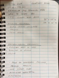
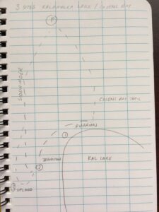
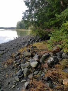
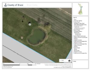
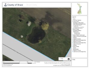
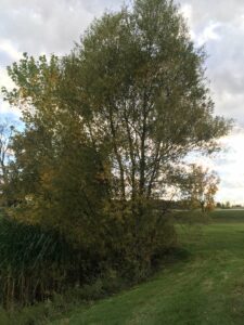
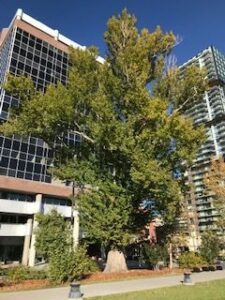
The three environmental gradients I am choosing to study in Cosens Bay include the riparian area of Kalamalka Lake, a transition zone between the riparian area and an upland area, and the upland area (Photo 1). Site 1 is the Riparian Area, Site 2 is the Transition Area and Site 3 is the Upland Area. On October 13, 2019 the three gradients were reviewed to observe the distribution, abundance and character of snowberry. On the day of the site visit, the temperature was approximately 7 degrees Celsius, cloudy with rain and observations were made between 9:00 am and 11:30 am.

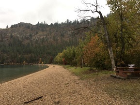
Photo 1. View looking north illustrating three gradients from Riparian to Upland.

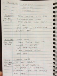
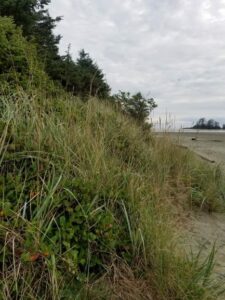
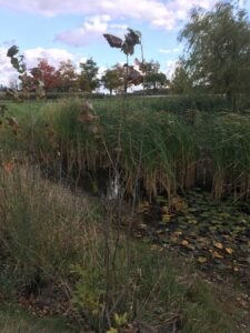
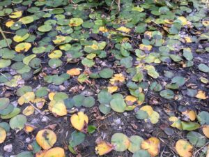
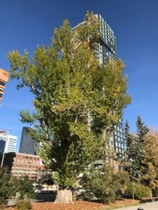
Site 1 (Riparian Area) is located approximately 10 m from Kalamalka Lake and snowberry is densely vegetated in shrub thickets along Cosens Bay Trail on the foreshore of Kalamalka Lake (Photo 2). The shrub appears relatively tall, with thick foliage with a large volume of berries. The leaves are bright green and the shrub appears to be thriving underneath a deciduous tree canopy of black cottonwood (Populus trichocarpa) and trembling aspen (Populus tremuloides) with dense shrub cover. The topography is relatively flat, facing south-west, with a wetland feature occurring upslope providing moist growing conditions.

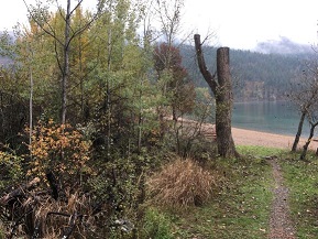
Photo 2. View of the Riparian Area with dense snowberry under a deciduous canopy.

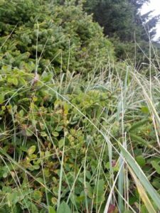
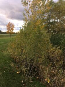
Site 2 (Transition Area) is located approximately 50 m upslope from Kalamalka Lake and snowberry is relatively sparse and appears shorter, with less foliage and less berry growth (Photo 3). The leaves are a lighter green and the shrubs were observed underneath a moderately dense canopy of ponderosa pine (Pinus ponderosa) trees. The topography is steeper than the Riparian Area and faces south east dominated by ponderosa pine and bluebunch wheatgrass (Pseudoroegneria spicata) with limited shrub coverage.

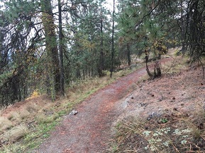
Photo 3. View of the Transition Area with sparse snowberry.

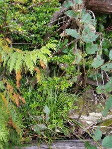
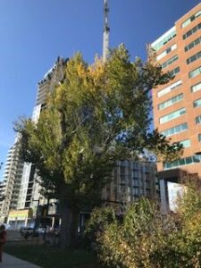
Site 3 (Upland Area) is located approximately 100 m upslope from Kalamalka Lake and snowberry is sparse to not present in this area (Photo 4). Shrubs that are present are small with less foliage and berry growth. The area is dominated by ponderosa pine, interior Douglas fir (Pseudotsuga menziesii), Saskatoon (Amelanchier alnifolia) and bluebunch wheatgrass. The tree canopy is open with little shrub cover. Other notable features in this area include relatively shallow soils with sporadic large boulders and the slope is steep, facing directly south.

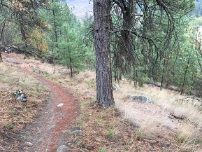
Photo 4. View of the Upland Area with little to no snowberry present.

In summary, snowberry was observed in dense quantities in flat, moisture receiving areas (Riparian Area) and sparsely vegetated to not present in steeper, dry sloped areas (Transition Zone and Upland Area).

The underlying processes that are may be contributing to the distribution and abundance of snowberry includes the hydrological cycle and moisture availability in soils. Based on my observations and the concept of limiting physical factors, water retention in the soil may be limiting snowberry to moisture receiving environments which is indicative of relatively flat topography.

One hypothesis to prove or disprove my observation is, “The distribution of common snowberry is determined by slope”. My prediction is “Common snowberry will be present in areas where slope is less than 20% grade”.

My experimental design would aim to empirically validate the pattern, that common snowberry distribution is limited to areas with less than 20% grade or that common snowberry distribution diminishes as percentage slope increases.

Based on my hypothesis that “The distribution of common snowberry is determined by slope”, one response variable could be the presence or absence of common snowberry which would be categorical. One explanatory/predictor variable could be the percentage slope, which would be continuous. Based on a categorical response variable and a continuous explanatory/predicator variable a logistic regression design could be utilised.

References:

E-Flora BC Electronic Atlas of the Flora of British Columbia [Internet]. 2019. Lab for Advanced Spatial Analysis, Department of Geography, University of British Columbia [cited October 14, 2019]. Available from: https://ibis.geog.ubc.ca/biodiversity/eflora/

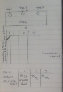
Field notes have been provided below:


Blog Post #3 – Ongoing Obs.

User:  | Open Learning Faculty Member: 


I revisited the park Oct 11, 2019 at 2:13pm. The temperature was 6°C and humidity at 42%. From my previous observations, the trees looked different in all areas of the park, some were decaying while others are still mostly green. Hence, I have chosen the study how the temperature, and especially the humidity from changes in weather, are going to affect the changes in certain trees. there are three deciduous trees, comparable in size and all quite bigger than the other trees, all located along the North side of the park.

Hypothesis: The colder and dryer the weather gets over the course of Autumn, the more the leaves of the trees will change.

Prediction: As the weather gets colder and dryer, then all the leaves in each of the three trees should change at approximately the same rate.

Response Variable: Amount of color change in leaves in each tree. It will be a continuous variable as the amount of color changed leaves from green to yellow is a % of all the leaves on the tree.

Explanatory Variable: Level of humidity. It is a categorical variable as humidity will be placed in low (< 30%), medium (30-70 %), and high (>70%) levels.

Tree 1

Tree 2


Tree 3

Blog8 Table and Graphs

User:  | Open Learning Faculty Member: 


Blog 8; Table and Graphs


October 12, 2019


For my field research study I created a table and a figure from the data I collected. When I collected the data I used two categorical variables. The first was the presence\absence of Hydrocotlye heteromeria in each of the quadrats I examined. The second categorical variable I used was wet\dry plot. I determined how many of the quadrats had the presence or absence of the species in each of the wet and dry plots. Since I am using categorical variables, and my study is a snapshot, natural experiment with 2 categorical variables I used a tabular method to determine my data.


I created an “Observed” data table including totals what the actual data I examined. I also developed an “Expected” data table and totals. I needed to create an expected data table to determine what I should have expected if the variables were unrelated. The “Expected values are what would be expected if the Null hypothesis were true and the variables were independent of one another. I then performed a Chi statistical test to determine if the relationship between Hydrocotyle and soil moisture levels was statistically significant. I determined that there is evidence that Hydrocotyle heteromeria is limited by soil moisture levels.


I also used the percentages of Hydrocotyle presence and absence that I found from each of the plots to create a figure. The figure is an easily identifiable way to quickly check how the counts and variables in the data table relate to one another.


The only problem I encountered when doing the table and the graphs was the fact that the course actually didn’t contain any material on how to process data information depending on which of the study methods we chose to use. I had to consult the professor of the course to determine the correct statistical test needed to analyse my study data. The table information and statistical testing was fairly straight forward after I completed the data counts. The outcome of the research is exactly what I had expected after reading literature. Hydrocotyle is limited by soil moisture levels. I didn’t take into account the nutrient levels in this study, but I would however like to learn more about their effect on this interesting species.