The data that has been collected is not overly surprising. I think the way that I have been collecting data is working well for this type of sampling/ experiment. My main issue has been trying to keep up with/ ensuring that I have not missed seeing a bee on one of the flowers within the bee garden.
The three sampling strategies used in the virtual forest tutorial are haphazard sampling, random sampling and systematic sampling. Haphazard sampling uses samples that are readily available, these samples are almost never random samples. Random sampling ensures that there is equal chance of being sampled. Systematic sampling avoids bias compared to haphazard sampling and is easier compared to random sampling.
Haphazard sampling had the fastest estimated sampling time. This is because there is less travel time between sample points.
The overall accuracy of the species that were more common was greater than the species that were less common.
The systemic sampling and random sampling strategy were the most accurate because the areas that were analyzed did not overlap.
I will be looking at the weather and the number of bees that visit the plants within the bee garden. Does the temperature seem to affect the number of bees? Or does the weather?
My response variable is the number of bees. My predictor variable is the weather. I believe these variables would be continuous because it is an infinite number between these two variables.
I am studying the “Bee Garden” that is located on the Thompson Rivers University campus in Kamloops beside the Ken Lepin building. It is a small garden with a variety of plants that are supposed to attract bees/ pollinators. There are a few benches that are near and two sets of stairs where people walk by. The first day that I visited the Bee Garden was June 2nd, 2019. That Sunday was relatively warm, within the twenties, and it was mid-day.
The three questions I have thought about are:
How many bees go to each plant?
Does the colour of the plant attract bees more? Or does the symmetry of the plant? (symmetry vs colour)
Does the change in weather seem to affect how many pollinators are out and about?
After going to talk to Dr. Lyn Baldwin about my hypothesis, and my questions, I decided to change my questions. Lyn suggested looking at the weather or the time of day, and then counting the number of pollinators. Therefore, my new questions would have to be:
Does weather seem to affect how many pollinators are out and about?
Does the temperature affect how many pollinators are out and about?
Does the time of day seem to change how many pollinators are out and about?
During the virtual forest tutorial, three sampling strategies were used to compare the abundance of different tree species throughout Middleswarth Natural Area. These strategies were the haphazard strategy, the random sampling strategy, and the systematic sampling strategy. I chose to sample by area not distance for the tutorial.
After completing the tutorial, it is estimated that the haphazard strategy was fastest for sampling (12 hours, 29 minutes) followed by the systematic sampling strategy (12 hours, 37 minutes), and the random sampling strategy taking the most time (12 hours, 42 minutes).
For the systematic sampling strategy, the percent errors for the two most common species were 20.2% and 31.2%, while the percent error for both of the two least common species was 100%. For the random sampling strategy, the percent errors for the two most common trees were 4.6% and 8.9%, while the percent error for the two rarest species were 100% and 50%. Finally, the percent errors for the two most common species using the haphazard strategy were 7.8% and 40.5%. The percent errors for the two most rare species were 4.6% and 100%. A percent error value of 100% occurred when no trees of those species were found during the sampling. From this, it can be observed that the lowest percent errors were found by using the random sampling strategy on the most common tree types, while the largest percent errors occurred when systematically sampling the least common species. Even more generally, the systematic sampling strategy yielded an overall percent error of 62.9%, the random sampling strategy yielded 40.9%, and the haphazard strategy yielded 38.2%. From these results, if one strategy had to be used, the haphazard strategy would yield the most accurate data on average.
Generally, as the abundance of a certain species decreased, the percent error increased. This indicated a decrease in accuracy, as the degree of closeness between measured and true values decreased. Conversely, the more accurate data was found in the samples of the most abundant tree types.The most accurate strategy for sampling the most common tree species was the random sampling strategy, and the most accurate strategy for sampling the rarest tree species was the haphazard strategy. It should be noted that the average percent error for the rare species was still much larger than the average for common species. Thus, it is important to understand the expected density and abundance of the species of interest to choose the sampling strategy that will yield the most accurate data. From this tutorial, it is evident that best strategy may not be the same for sampling all tree types. Ensuring the proper strategy is used will allow for sampling data to best represent the population data.
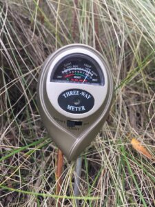
The purpose of this fieldwork was to observe aspen trees, Populus tremuloides, located in Whispering Woods. One of the environmental gradients present at this location is a 12m change in elevation from the bottom to the top of the Woods. Therefore, I chose to observe health attributes of P. tremuloides trees located at the bottom, middle, and top of this hill. The specific attributes I observed were leaf colour (percent of primarily yellow leaves on the trees), soil moisture (measured using a HoldAll® Moisture, Light, and pH Meter™), and soil pH (also measured using a HoldAll® Moisture, Light, and pH Meter™). Soil moisture and pH measures were taken 20-30cm from the base of the tree. Additionally, I looked at general differences in the distribution, abundance, and character of these trees located at the bottom, middle, and top of the hill.
HoldAll® Moisture, Light, and pH Meter™ reading moisture level of soil near a tree at the bottom of the hill
Observations recorded in field journal describing differences in leaf colour percentage, average soil moisture levels, average pH levels, and density of trees located along the gradient of the hill slope.
Observations from field journal measuring the soil moisture level and pH of n=10 trees chosen using convenience sampling for the bottom, middle, and top of the hill. Average soil moisture and pH also calculated, with rankings shown.
As indicated from the field journal documentation, there were character differences present including the percentage of yellow leaves, soil moisture, and soil pH of the 30 trees sampled (10 from each level of gradient). The bottom of the hill contained trees with almost completely green leaves, a higher average moisture, and a medium average pH. The top of the hill contained trees with primarily green leaves on its West side, and primarily yellow leaves on its East side. Further, trees on the top had the lowest average soil moisture, and most alkaline average soil pH. Trees located in the middle of the hill had a combination of characteristics from both.
Additionally, I observed differences in the abundance of trees, as the top NW contained the densest area of trees, while the bottom SE corner contained the least. These dense trees were also smaller in size on average. The distribution of yellow coloured leaves also was a clear finding, with primarily yellow-leaved trees located on the East side, and primarily green-leaved trees located on the West side for both the trees sampled from the middle and top of the hill. Another important note is that there were not enough trees to sample from the bottom SE corner relative to the width of the hill, so samples taken from the bottom of the hill were taken from trees all on the SW side.
From these observations, I have compiled a hypothesis and a prediction. It is important to note that in this stage of my Field Project, I am choosing to define the “health” of these trees as green leaves, high soil moisture, and a neutral soil pH. As the Fall season progresses, I hope to include other relevant indicators, such as rate of leaf loss, and perhaps water infiltration rate.
My hypothesis is that there is a significant difference in P. tremuloides health (based on the definition above) among trees located along the elevation gradient of Whispering Woods hill. My null hypothesis would therefore be that there is no difference in P. tremuloides health among trees located along the elevation gradient of Whispering Woods hill; any difference is due to chance alone.
Based on this hypothesis, I can make certain predictions regarding the attributes of health I have chosen. I predict that trees located at the bottom of the hill will have a better overall health, indicated by a higher average green leaf percentage, higher soil moisture, and a neutral soil pH. Conversely, I predict that trees located at the top of the hill, on average, will have a worse overall health, indicated by a lower green leaf percentage, lower soil moisture, and a more alkaline soil pH. These predictions are based on my previous knowledge of what plants require to grow optimally.
From these predictions, the response variable would be indicators of tree health (soil moisture, percent green leaves, soil pH) which is a continuous variable. The explanatory variable would be the position of the tree on the hill (bottom or top) which is a categorical variable.
My field data collection began when I revised my plots to include 2 separate plots of wet and dry soil. I created a field data table similar to the activity in Module 3. I set up the table to include the 6 replicates I have chosen; Hydrocotyle Heteromeria, Trifolium repens, Glechoma hederacea, Bellis perennis, Poa pratensis and Elymus repens.
My design is a Logistical Regression experiment as I am determining a categorical predictor variable. The predictor variable for the hypothesis is soil moisture. I have determined areas which contain high levels of soil moisture and areas of less soil moisture using a ‘soil moisture meter.’ According to Gotelli and Ellison (2004), am hoping to determine the “effects of X on Variable Y.” My experiment will help me determine if the effects of moisture variable ‘X’ limits the abundance of Hydrocotyle plant ‘Y’.
I have not had any trouble implementing the Logistical Regression sampling design, on the systematically placed transects. My data table has a categorical predictor of ‘absence or presence” of the replicates in each quadrate in the two sample plots. The only issue that I had not accounted for was the fact that it was so time consuming. Looking at 16 quadrates in two 5x5m sections to determine each species took me hours.
To decrease the chances that the experimental data results may not be a representation of the actual patterns occurring, I will have a large scale area to sample, greater than 1m2 (Gotelli 2004, Englund 2003).
I am performing a natural experiment in which the two plots are in natural settings and have not been manipulated. I am performing a snapshot survey of the plots (in the month of September) instead of a trajectory experiment which would be done over time and years (Gotelli 2004). Snapshots work well because the replicates are more likely to be independent of one another as compared to the trajectory experiments (Gotelli 2004).
I will be using 6 replicates which are the 6 most common species found in my lawn experiment. Using the “Rule of 10” I have systematically set up 4 transects in a North/South and East/West direction to give me 16 study plots in each of my 2 designated “high moisture content” and “low moisture content” areas. The quadrate size is 17x17cm, which will ensure that the samples are far enough apart to be independent. Both of the plots are homogeneous in climatic conditions. I don’t not need a control group as I am not manipulating the experiment, I am surveying the natural landscape.
Grain: Smallest unit of study = the absence or presence of the replicate in the 17x17cm quadrate
Extent: Total area encompassed by all sampling units = 2.7m2 of sampling area
Citation
Gotelli and Ellison. 2004. A primer of Ecological statistics. Chapter 6; Designing a Successful Field Study. Web. Accessed TRU.
Englund, G. and S.D. Cooper. 2003. Scale effects and extrapolation in ecological experiments. Advances in Ecological Research 33: 161-213. Accessed TRU.
Looking back at the original design of my field research, I recognized a problem getting accurate representation of the mean grass distribution. The grass was naturally distributed in clumps which meant a smaller number of samples would likely result in a misrepresentation of the cover. I made the change to add more transects after the initial collection of data, but I still feel the number of transects could have been doubled to property represent the mean distribution. Prior to taking this course, I took GEOG 3991 Climate Change. I learned about the many negative impacts of climate change on our sensitive ecosystems caused by anthropologic sources. Ecology has deepened my appreciation for how ecologists meticulously gather data which can be used as evidence of the impacts of climate change. I have a greater understanding of the processes that go into research, the time that is in involved in accurately collecting data, as well as the other confounding factors that need to be accounted for.
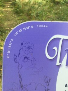
I have chosen to observe a small deciduous forest, approximately 150 square metres in size, located at 51°6’14”N and 114°8’21”W, just outside of the NW Calgary Dr. EW Coffin Elementary School limits. This city park was adopted by the elementary school through the Adopt-A-Park program, but otherwise holds no designation. I visited this site on September 16, 2019 from 3:15pm to 3:50pm. The weather was 16°C and mainly sunny with some cirrus clouds.
Coordinates of Whispering Woods on informational sign
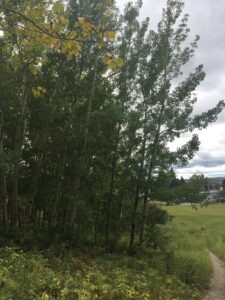
Large, green aspen trees on South face bottom of hill
The forest is located on a hillside, with the elevation gain of about 12m, from an altitude of 1130m at the bottom of the forest limits to 1141m at the top. It is primarily made up of aspen trees, both large and small. Beneath these trees sit a variety of flowering plants, berry bushes, thistle, mushrooms, and smaller leaved trees. The floor of the forest is comprised of smooth, brome grass. Large aspen trees are found on the South-West bottom edge of the hill, along with the long, native grass, the thistle bushes, and the mushroom patches. The centre of the forest is more clear of aspen trees and is comprised mainly of smaller bushes. The top of the forest contains densely-packed aspens, none of which are as large as those on the bottom face. Throughout the forest are multiple gravel paths, grass foot-paths, and informational signs. An amphitheater is also located on the North side at the top of the hill. Small, bee-like pollinators were present on the flowering plants, and mosquitoes were identified.
Tall, native grasses on South face bottom of hill
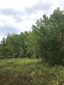
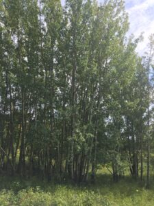
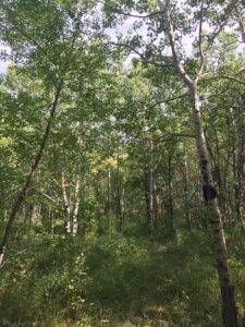
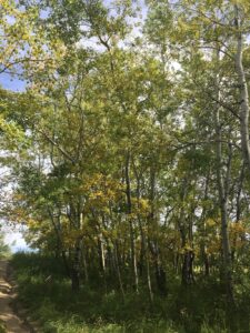
Dense aspen forest near top of hill
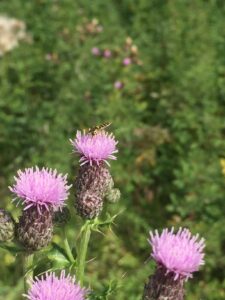
Pollinating bug on thistle flowers
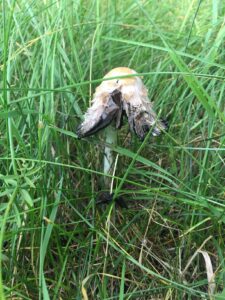
Mushroom towards bottom of hill
There are certain observations that caught my attention during my visit. Dandelions seemed to have taken over the centre clearing of the forest, leading me to my first question of interest: What has allowed for this dandelion take-over in the centre forest, and why are they so contained to this area? I also noticed that the aspen trees on the South face were very green, and much larger than the others. Finally, I observed that, on average, the smaller aspen tree leaves appeared to be much more yellow than the leaves on the larger trees. I have multiple questions related to these observations. For one, what factors are causing the smaller trees to turn yellow faster than the larger trees? My final question of interest is less based on an observation I noticed during this visit and more a question for the future: Are there differences in the rate of leaf colour change, and then leaf loss, in the trees located on the top of the hill versus on the bottom? In other words, how does tree position on a hill affect its health as the Fall season progresses with regards to colour change and leaf loss?
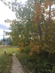
Leaves changing colour on smaller aspen trees
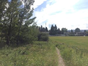
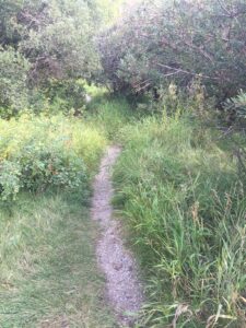
Gravel path to top of hill
I look forward to narrowing down my subject for this research project, as this forest offers many questions waiting to be answered.
The source of scientific information I chose comes from the TRU library. It is A conceptual framework for understanding the perspectives of the causes of the science-practice gap in ecology and conservation conducted by Diana Bertuol-Garcia, Carla Morsello, Charbel N. El-Hani, and Renata Pardini; all of who are considered experts in the field as they are employed by universities. This, along with in-text citations and a list of references confirms that the paper is academic. In the acknowledgement section, the author’s thank the two anonymous referees who reviewed the paper, making it peer-reviewed. The article includes methods and results sections making it a research paper. In all, the source is academic, peer-reviewed research material. The link for the source is below:


 This image demonstrates that the author’s are experts.
 This image demonstrates that there are in-text references and that the article contains a method’s section.
 This image demonstrates that there is a results section included.
 This image shows that two anonymous referees reviewed the paper.
 This image demonstrates that there was a list of references included.