Recent Posts

Post 3: Ongoing Field Observations

User:  | Open Learning Faculty Member: 


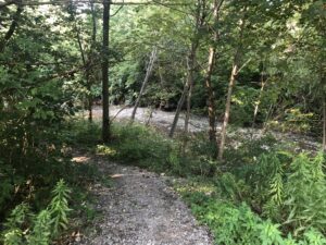
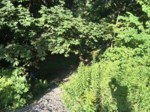
The organism that I have chosen to study is the perennial plant Canada goldenrod (Solidago canadensis). As mentioned in a previous post, I observed that the height and density of this plant varied depending on its location. In some areas the plants were completely in the shade, while in other areas they were exposed to direct sunlight. Therefore, the environmental gradient I have chosen is the degree of sunlight exposure. The three locations along the environmental gradient I have identified are areas where the goldenrod has access to direct sunlight, has only partial sunlight exposure, and is completely in the shade. I have labelled these areas as high, moderate, and low levels of sunlight exposure, respectively. In the areas of low sun exposure, the plants had the lowest density, appeared to be the shortest, had minimal flowering buds, and were sparsely distributed. In the areas of moderate sun exposure, the plants appeared to be slightly taller than the plants in the low sun exposure area and had greater plant density. In the areas of high sun exposure, the plants were the tallest, appeared to have the greatest density, and a majority of the goldenrod plants exhibited flowering buds.

Hypothesis: Level of sunlight exposure affects the growth of Canada goldenrod (Solidago canadensis).

Prediction: If this hypothesis is true, then it is predicted that the height of Canada goldenrod will increase with the level of sunlight exposure.

Response variable: Plant height. This is a continuous variable as it is measured on a numerical scale in inches.

Prediction (explanatory) variable: Level of sunlight exposure. This is a categorical variable as we are observing, not measuring, the categories low, moderate, and high sunlight exposure.
    

Post 2: Sources of Scientific Information

User:  | Open Learning Faculty Member: 


Liu, Y., Dawson, W., Prati, D., Haeuser, E., Feng, Y., & van Kleunen, M. (2016). Does greater specific leaf area plasticity help plants to maintain a high performance when shaded? Annals of Botany, 118(7), 1329-1336. doi:10.1093/aob/mcw180   

The source I found is an article published in the journal Annals of Botany. I classified this source as academic peer-reviewed research material. The article was written by experts in the field of biology and plant sciences, who are associated with numerous reputable universities. The article contains frequent in-text citations from various sources and journals as well as a list of literature cited at the end of the text. I classified the article as peer-reviewed academic material since the authors acknowledge two anonymous referees who reviewed the article prior to publication. Finally, I identified the article as research material, since it contains a Materials and Methods section, as well as a Results section outlining a research study.


Post 1: Observations

User:  | Open Learning Faculty Member: 


The location that I have chosen to study is a section of land adjacent to Mimico Creek, which is situated between two residential streets in west Toronto, Ontario. The creek extends a total of 33km in length, however, I will be observing only a portion of the land approximately 20 m long x 15 m deep. The creek water is approximately one meter below the creek bank, and most of the vegetation exists on elevated area. The area surrounding the creek is on a gradual slope upwards away from the water that contains various types of different green vegetation with minimal flowers. The vegetation includes various perennial plants, grasses, weeds, and trees. The density and height of the vegetation varies across the study area, depending on the distance from the creek and varying sunlight exposure due to shade provided by trees. The ground consists of scattered grass, dirt, and small rocks. There is a man-made footpath that runs adjacent to the creek.

I visited the observation area at 12:00 EST, on August 5, 2019. The weather was a mix of sun and clouds, with a temperature of 25°C and wind speed of 34 km/h.

While visiting the site, I noticed that there was one dominant plant,Canada goldenrod (Solidago canadensis). I observed that the height of the plant varied significantly depending on its location. It appeared to be shorter in the shaded area directly next to the creek, and taller approximately 10 m from the creek in the elevated area situated in direct sunlight. Additionally, there was more plant growth (species density) in the elevated area with greatest exposure to sunlight. Thus, this presents a few potential topics of study.

Three potential study questions:

  1. What is the effect of distance from the creek/elevation on plant height and density?
  2. What is the effect of sunlight on plant height and density?
  3. What environmental or anthropogenic factors affect the observed distribution of plant species?


Blog Post 9: Reflections

User:  | Open Learning Faculty Member: 


In hindsight I wish I would have broadened my sample size as I was very limited. However, I believe I was able to gather enough data to conduct my experiment and felt that, while it was a simple design, it was a straightforward enough so that I could digest what was happening at the pace I was comfortable with. For the future I hope to become more confident in creating a design that can be expanded upon and not remain so limited.

Blog Post 4: Sampling Strategies

User:  | Open Learning Faculty Member: 


I started the tutorial using the area-based model for all three of the sampling techniques. There was not too big of a difference between the duration of the samplings, but I found the fastest of the three techniques to be using the haphazard technique (14 hours). I found that the haphazard technique yielded the more accurate sampling error when it came to rare species, whereas the systematic approach was better in determining percent error results for the two common species. In terms of effectiveness of techniques, the haphazard provided better results, compared to the systematic and random approaches.


Post 9: Field Research Reflections

User:  | Open Learning Faculty Member: 


Since the field experiment that I designed and based my research around was fairly straightforward and simple, I did not have many difficulties in carrying out data collection or analysis. I did not make any changes from my original design that I drafted back in April as the abundance of mature western redcedar trees in the research area did not change between the spring and late summer when my analysis and report were concluded. There are aspects of field work that I had never considered before completing this project, and it definitely allowed me to appreciate the meticulous record keeping that must be done when large experiments and observations are being conducted. The work that is done by ecologists to preserve mature stands of forest is incredibly important and this research has made me acknowledge just how much work and dedication the ecologists have put into the conservation of the natural world and our understanding of it.

Blogpost 8: Tables and Graphs

User:  | Open Learning Faculty Member: 


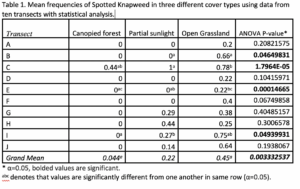
Organizing my data into my table was not difficult, only time consuming. Calculating mean values was quick and easy but conducting the statistical analysis was time consuming. I definitely had to do further research on the t-tests (and therefore also the necessary F-tests) for determining significance between means after the ANOVA test was completed. While this took time, it made sense in the end and I feel that I’ve presented all relevant statistics by doing so.  The trend that I’ve noticed with the grand mean is that the canopied forest and the open grassland have significantly different frequencies of Spotted Knapweed. The partially lit open canopied forest is not significantly different from either of the other two cover types when looking at the grand mean; when looking at individual transects this may not be the case (see below). It would be interesting to see how these results would compare to a study with more samples to have an even better representation of the frequencies; additionally, it would be interesting to see data from studies of this nature at other sites.

Blog Post 5: Design Reflections

User:  | Open Learning Faculty Member: 


Blog Post 5; Design Reflections


My sample strategy was Systematic sampling which was easy to design. I found a few problems with the design and statistics sample sizes. Statistically speaking, “the sample should be no more than 10% of the population” (De Veaux et. al, 2014, p.411). To obtain a sample of only 10%, I needed to create a smaller quadrate, decrease the amount of transects of increase my plant coverage.

I decided to divide my single plot into 2 separate plots. Both plots will be 5m x 5m. One which contained soil with a large amount of moisture and one which contained soil with low moisture. To make sure I had less than 10% of the population within my sample units, I will place 4 transects East/West and 4 North/South. This also allows me to obtain 16 samples in each plot, which is larger than the required 10 samples per area. My quadrate must then be 17centimeters x 17centimeteres to give me a total of 2.72m2. This puts my sample under the 10% of the population.

I also altered the plots so that the sample areas were not on the boundaries, and did not overlap between the “Wetter” and “Drier” areas. I will continue to use the Systematic sampling techniques as it worked well for my data documentation.

The modification will help me to easily distinguish between the two areas of moisture, while allowing to be obtain a proper sample amount in comparison to the total population.


Citation

De Veaux, D., Velleman, P., Bock, D. Intro Stats Fourth Edition. Copyright 2014, 2012, 2009. Pearson Education, Inc. Upper Saddle River New Jersey.

Blog Post 9 – Field Research Reflections

User:  | Open Learning Faculty Member: 


I did not have any issues implementing the design, so I did not have to make any changes to the design. After completion I have started to consider that it would have been good to choose a location that doesn’t have as many anthropogenic influences (i.e. a wild field, not municipally owned). I believe that the interactions such as the competition the grass adds because of lawn mowing and disturbances caused by both humans and domesticated animals may have skewed some of the results. These were things that I did not realize initially, but I believe that with time and experience these would be factors that I would have picked up on sooner. I think that this first personally designed ecological study was an eye opener and has given me my first real good glimpse into what working in the field could be like. Engaging in this practice of ecology and designing this field research has greatly increased my appreciation of the entire study of ecology and everyone who partakes in it. I think that I was very unprepared for how much thought goes into these studies and also how much actual physical effort does too. My fieldwork was in no way large scale and I was exhausted and my neck hurt from counting all the clovers. I have a great appreciation for ecologist’s work ethics and perseverance.

While conducting my research and looking for relevant journals and papers I came across this article and found it very interesting. This idea of “clover lawns” is what sparked my interest into researching Trifolium repens. 

Smith, L. S., and M.D.E. Fellowes. 2013. Towards a lawn without grass: the journey of the imperfect lawn and its analogues, Studies in the History of Gardens & Designed Landscapes, 33(3): 157-169. doi10.1080/14601176.2013.799314

Blog Post 8: Graphs and Tables

User:  | Open Learning Faculty Member: 


Creating a graph to represent the collected data went smoothly as it was easy to represent the total amount of sunlight graphically for each day I spent observing. I created a separate graph for the individual days I collected data, and then combined them in a bar graph that represented the combined amount of time for each marking. Once again, the data supported my initial hypothesis as the markings that contained Seedling 2 averaged the most sunlight exposure. The markings that contained Seedling 1 averaged the least exposure whereas the markings containing Seedling 3 was only slightly lower than that of Seedling 2.