Recent Posts

Blog post 9: Field Research Reflections

User:  | Open Learning Faculty Member: 


The fieldwork this class has allowed me to perform was very engaging and motivating in my biology undergrad journey. I very much enjoyed applicating of all this theory on field research and biological work that I have been studying and fantasizing about. Conducting my own study was a challenge on its own as it was the first time I had ever done a full project of this sort fully by myself. I loved the freedom of choice we had in the beginning as t what we would be studying. This freedom of choice actually made it challenging as with my very limited experience in research, I had a few flaws in my initial plans. Per example, my first ideas were way too grandiose and hopeful. I quickly understood the extent of the work necessary to drive research in the field. What I loved about this, is that it motivated me for future potential larger-scale studies in my career instead of simply discouraging me. I lowered the scale of my research here in order to create quality work but I simply cannot wait to participate in larger, more important work. Another flaw my initial plan had was the lack of a control in my idea of assessing the gradient in flower abundance. I have greatly learned from this experience and as I said cannot wait or te next. I greatly appreciated the systematic way ecological work is done. I believe that to understand such an intricate system that is a community or an ecosystem, empirical work is necessary to formulate a more informed guess as to what is really going on. I think the scientific method is a great way to understand greater scheme problems and ecology showed me a fun way to systematically work on a system as complicated as a field full of seemingly random flowers. I love finding patterns!
Blog Post 8: Graph

User:  | Open Learning Faculty Member: 


I was having trouble compiling all of my data within only one graph. It seemed as I had too much information to include in the graph. I then decided to combine 4 graphs (A, B, C, D) into my one Figure. By having those four graphs separated but put together in one figure, it was very easy to compare them all. The proximity and arrangement allowed for an easy and quick assessment of all four data that is essentially the same experiment but for four different species. I found that it illustrated well the differences between species. Some basic technical difficulties were met when I was trying to combine all four graphs and axis titles into one figure. I ended up combining them all through powerpoint into one image that I then introduced into my word document. This technique facilitated the whole process by unifying all my elements.

My data put into graphs actually showed me that there was an increase in flower abundance as one gets away from the beach as I hypothesized. Though, I had not observed the fact that abundance declined within the last two or three subsamples along my transects. This new discovery would definitely be worth studying to understand if perhaps another gradient or ecotone is present as the field gets closer to the highway.

Blog Post 5 – Design Reflections

User:  | Open Learning Faculty Member: 


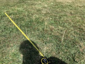
When implementing my sampling strategy, I found that the process took much longer than expected. Based on the experimental design I chose I utilized stratified random sampling because I needed to have a plot from each “location” along my gradient. I wanted to use an adequate sized plot so I decided to divide my plots into 25 smaller quadrants in an attempt to be more accurate and ease the process of counting the clovers. Unfortunately, the act of splitting the plots took a long time. However, I do think it was beneficial to use the 12 inches by 12 inches quadrants.

The data collected was not overly surprising, I was correct in expecting the highest abundance to be found in the no shade area. However, I was surprised that the clovers observed in the partial shade location were noticeably larger than the clovers from all other locations. They did also seem to be healthier and thriving more compared to the clovers found in other locations.

My only difficulty in implementing my sampling strategy was purely the duration. Although it was not difficult both the counting of the clovers (which were more numerous than I had thought) and the plotting and measuring of the quadrantswere very time consuming.

I will continue to use the same technique because I believe it yielded the most accurate results and feel confident with how my data collection went. If I was to use larger quadrants it would increase my chances of error.

Blog Post 9: Field Research Reflections

User:  | Open Learning Faculty Member: 


At the beginning stages of my field research project, I took a day or two to choose my research topic and my first observations of the area went smoothly. Since my sample area was located in my backyard, time was never a factor with my field data collections. However, the further I got into this project, the more difficulties I faced. An important lesson that I learned was that not all potential explanatory variables will be easily collected, examined or measured. I found this when I was deciding on how to represent and measure the effects of pH on Common Fern Moss percent cover. I was unable to easily measure the pH of the dead and healthy portions of grass and I was unable to think of a way to represent this data while displaying the relationship between pH and absence/presence of Common Fern Moss. I had to work around this problem by resorting to research articles touching on this relationship instead. In terms of the design of my project, I had to make a few adjustments along the way which weren’t too problematic. For example, I changed my quadrat size from 1m2to 0.25m2in order to minimize the amount of overlap between quadrats, and by doing this I had to recollect data on the first five quadrats I placed in the yard (which wasn’t an inconvenience as I had to collect data on 10 additional quadrats anyways…). Enrolling in this course and carrying out this research project on my own has not only altered my perspective on this practice, but has also increased my appreciation for the time and effort put in by ecologists to understand ecological processes and patterns. Conducting a research project isn’t easy, and from my experience, I believe it is a task that requires quite a bit of patience and an optimistic and open mindset.

Blog Post 4 – Sampling Strategies

User:  | Open Learning Faculty Member: 


For the virtual forest tutorial, I used the area-based model for my systematic, randomized and haphazard sampling of vegetation. The technique which required the least amount of time was the haphazard method. However, all sampling techniques had very similar sampling times around 12.5 hours. For the two most common species the systematic approach gave the best percent error results, while the haphazard sampling gave the worst results. Alternatively, the percent error for the two rarest species was best using the haphazard sampling technique. It seems that the systematic approach is more useful for large amounts of common species, while the haphazard sampling was more accurate for the rarer species. Based on the percent error data for all six species the haphazard method presented the best results on average, followed by the systematic and the randomized approach.

Blog Post 3 – Ongoing Field Observations

User:  | Open Learning Faculty Member: 


I revisited my chosen area on August 4th 2019 at 13:37. I have decided to conduct my field research study on the plant species Trifolium repens (common name White Clover). Specifically, the distribution and abundance of Trifolium repens across the three locations I identified along the environmental gradient.

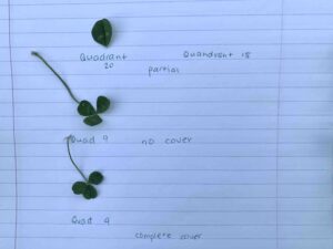
Trifolium repens is a small plant which appears to mainly grow in clusters. Most often they are found to have three balloon shaped leaves which are approximately 0.5 – 1 cm long and their stem is approximately 1-3 cm long.

The 3 locations I chose each differed in the amount of shade/coverage that was provided to the clovers. The 3 locations were as follows; shade, no shade and partial shade. The clovers did grow in each of the three locations, however there was a distinct difference in the abundance of clovers across the locations. The “no shade” location appeared to have the highest abundance of clovers, the “shade” location had the lowest abundance and the “partial shade” area was in between.

Furthermore, in the “partial shade” location I noticed that the phenotypic expression of the clovers differed. The clovers I studied in that location had much larger leaves, approximately 5mm longer than the leaves found on clovers in other areas. At a far glance it appeared that the abundance was highest in this location, however with closer inspection I noted that apparent abundance was most likely due to the larger clovers.

Hypothesis : Plants need sufficient access to many natural resources, including sunlight. With lack of sunlight the plants cannot thrive.

My prediction is that Trifolium repens will grow in higher abundance in sunlight, therefore the abundance will be highest in the “no shade” location.

One potential response variable is the abundance of Trifolium repens (continuous). One potential predictor variable is the amount of access Trifolium repens has to sunlight (categorical).

Based on the experimental design tutorial I deduced that my experimental design would be classified as ANOVA

Post 8: Tables and Graphs

User:  | Open Learning Faculty Member: 


I did not have any difficulties summarizing my abundance data in a simple bar graph, categorized by the three kinds of soil upon which my hypothesis is based. I graphed the relationship between the soil texture at each site along my environmental gradient and the abundance of individual trees sampled. The outcome supported my hypothesis that western redcedar trees would dominate areas of loamy soil that have better moisture-retaining properties than the sandy sites. The bar graph neatly summarizes the presence and absence of the three main species of the area: western redcedar (Thuja plicata), Douglas fir (Pseudotsuga menziesii), and ponderosa pine (Pinus ponderosa). The data did not reveal anything unexpected, but it inspired me to look into why western redcedar was completely absent from the sandy site (site 1) but was represented in the silty site (site 3). This prompted me to research competition between species in the interior cedar-hemlock biogeoclimatic zone, specifically between shade-tolerant and shade-intolerant species. It also inspired me to think critically about the overlapping niches of each species and how their evolutionary history has played a role in the spatial distribution of individuals within a mature stand.

Blog Post 2 – Sources of Scientific Information

User:  | Open Learning Faculty Member: 


I chose an article from the American Journal of Botany titled “Freeze‐induced cyanide toxicity does not maintain the cyanogenesis polymorphism in white clover (Trifolium repens)”. I sourced it from the University of Victoria’s online library database.

https://bsapubs-onlinelibrary-wiley-com.ezproxy.library.uvic.ca/doi/abs/10.1002/ajb2.1134

The article can be classified as academic, peer-reviewed research material. It was written by four experts in the field, all of who hold PhDs and are in the Department of Biology at their respective universities. The article also includes many in text citations and a complete bibliography. On page 1230 in the acknowledgments section it is noted that the article was peer-reviewed by 2 anonymous reviewers. Finally the article can be easily determined to be research material rather than review material by the presence of both a “Methods” and “Results” section.

Blog Post 1 – Observations

User:  | Open Learning Faculty Member: 


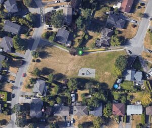
The area that I have selected to observe is a small community park near my house that is frequented by both humans and animals. I visited the area on August 3rd, 2019 at 14:01. The temperature was 18 C˚ and the weather was sunny with a light breeze. The park is situated in a residential neighbourhood in Victoria, BC. The park is mostly open flat grassland with trees growing in some areas. The size of the park is approximately 0.32 hectares (this information was sourced from the district of Saanich website).


I identified roughly three different stratums; open grassland with no shade and no trees, an area with large deciduous trees and constant shade and an area with smaller trees which provided some coverage/shade. I observed the difference in organisms which grew in the different stratums. Overall, the dominant species were clovers, grass and two different species of deciduous trees.


3 questions that could form the subject of the project


  • In what ways does the proximity to a residential area effect the species diversity and richness?
  • What causes the clovers to grow in clusters rather than dispersed throughout the park?
  • What effect do the different trees/shade have on the organisms which live below?


Blog Post 4: Sampling Strategies

User:  | Open Learning Faculty Member: 


Adrienne Burns

August 21, 2019


The first sampling method I conducted was the ‘Area; Systematic” approach. I choose one randomized number ‘y’ axis, and received my subsequent data from adding 10 to each of the ‘x’ axis and alternating between the randomized number and ‘y+10’. The density data from this sampling method has some very accurate of methods for certain species of trees, but very inaccurate data for others. When comparing it to the ‘Actual density’ data, for example, the actual density of Sweet Birch was 117.5, and sampling density found 116, and for White Pines species, the actual density was 8.4 and the data showed a density of 28.0. I found it interesting that for the species Striped Maple, this method did not count any of the trees. The density for Striped Maple was 17.5 and this method accounted for 0.0. This type of sampling didn’t correctly depict the distribution of tree species over the entire forest area. Also, the ‘Area; Systematic’ method took a long time to complete. It took 12 hours and 35 minutes to complete the sampling.


The second method was the ‘Distance; Random’ sampling technique. This method had given me 24 random ‘x, y’ axis to sample. It was the fasting sampling method which took 4hr 38minutes. This would be the preferred method of sampling if the ecologist had time constraints. Along with the first method this one also showed varying correctness for the distribution of the trees. For example the actual Hemlock density was 469.9 and the data showed a density of 445.1, but for the Red Maple the actual density was 118.9, but the data showed 145.2. Of all 3 of the sampling methods I used, the ‘Distance; Random’ technique was the most accurate especially with regards to frequency.


The last method, ‘Area; Haphazard’ took the longest timeframe to complete 13h and 1minute. It also had the largest variation in results. For instance, Eastern Hemlock actual density was 469.9. Both ‘Area: Systematic’ and ‘Distance; Random’ data were close in proximity to 440.0 and 445.1, yet the ‘Area; Haphazard’ showed 669. As it had the largest variation and the longest timeframe, I would need to seriously consider I was going to use this method.


None of the methods were very accurate. All had some tree species data that was accurate, and others that were far from the actual data.


Error Percentage Eastern Hemlock


‘Area; Systematic’

(440-469.9)/ 469.9*100 = 6.36% Error


‘Distance; Random’

(445.1-469.9)/469.9*100 = 5.28% Error


‘Area; Haphazard’

(664.0-469.9)/469.9*100 =41.31% Error


Error Percentage White Pine


‘Area; Systematic’

(28-8.4)/8.4*100 = 233.33% Error


‘Distance; Random’

(9.7-8.4)/8.4*100 = 15.48% Error


‘Area; Haphazard’

(4.0-8.4)/8.4*100 = 52.38% Error