Recent Posts

Blog Post 8: Tables and Graphs

User:  | Open Learning Faculty Member: 


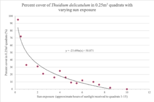
Above is the table I submitted for the fifth small assignment submission. It plots the relationship between the percent cover of Common Fern Moss, Thuidium delicatulum, and the degree of sun exposure in my yard. In order to create this graph, I had to measure the sunlight intensity of all quadrats (1-15) for every hour starting at 6:00 am and ending at 7:00pm on July 26th, 2019. Then, I sampled each individual quadrat for percent cover of T. delicatulum. I had some difficulty trying to categorize and separate each quadrat by the number of hours of sunlight received throughout this 13-hour time period. I eventually decided to basically approximate the relative amount of sun exposure received by each quadrat and used these values for the domain of this graph. When I put the graph together, I was very pleased to see that it follows my prediction (minus some outliers). I originally suspected that the graph of these two variables would be inversely proportional, and this graph mimics that trend.  One of the outliers located at point (4,25) really stuck out to me because this quadrat happens to be located in a section of my yard in between the Japanese Lilac Tree and the Columnar Aspen. This area receives minimal sunlight and I recognized the soil in this area to be relatively moist when I was sampling in Module 2. Being that it is too difficult to go about sampling and representing soil moisture with the limited tools and resources I have at home, my best bet in inquiring about this specific observation would be scientific articles on this subject. I am curious to see if there are any scientific articles/studies out there that touch on the relationship between soil moisture and moss abundance. This would help for further exploration and answer a few questions I have going forward.

Blog Post 3: Ongoing Research Material

User:  | Open Learning Faculty Member: 


Blog Post 3: Ongoing Research Material

Adrienne Burns

August 20, 2019


I have decided to do my research field study on the plant species Hydrocotyle heteromeria (Wax weed or Pennywort). I found it in a large patch around a wet soil area, underneath the mature Pyrus communis (pear tree). There were only a few areas I spotted with Waxweed species in large quantities, but perhaps with the field research project I may find smaller patches within the grassy areas. After I had completed a Tru.ca Library and internet research, it sounds as if the plant species prefers moist areas and grows in areas of yards, golf greens or forests that do not have well drained soil.

I found that by documenting the observable gradient of the landscape (attached photos), the plant species is clustered around areas 1 and 2. Both of the first two selected sites are in areas of lower soil levels. I notice that in area 1, where I first noticed the large clusters of Pennywort, there are small pockets of even lower soil levels around the base of the Pyrus tree. The Hydrocotyle heteromeria is found in large abundance in these pockets. In observation region 2, there is still large amounts of the plant found, but it looks as though there is a decreased amount of large clusters. It seems as though the plants are clustered around the base of the tree. There could possibility be a symbiotic relationship with the tree or the plant may prefer nutrients received closer to the mature tree. The nutrient level in the center and drier area of the landscape may differ from the nutrient level near the tree, especially because there are many large trees on the non-study side of the fence (approximately 4 feet from the location of found Waxweed). In both observational regions 3 and 4, there was no sign of the species, so distribution and abundance has decreased drastically.

I believe that these pockets of lower soils levels catch and contain more water. There would be an abundance of water especially around the base of the tree as the area receives less sunlight, and the lower soils levels would accumulate more water. There would also be an accumulation of water in areas 1 and 2 because of the winter water run-off from the tree.


Hypothesis: The distribution of Hydrocotyle heteromeria in the Christchurch New Zealand backyard landscape is limited to areas of soil with high moisture content. My

Prediction: H. heteromeria is seen in areas of high moisture and the plants abundance decreases at the soil becomes increasing dry.

Prediction Variable: Soil moisture. High moisture content or Low moisture content is a Categorical Variable.

Response Variable: Plant numbers decrease as soils moisture decreases. The sample units would be Categorical as “absent or present.”


Blog Post 2: Sources of Scientific Information

User:  | Open Learning Faculty Member: 


Blog Post 2: Sources of Scientific Information

Adrienne Burns

August 19, 2019

Citation

Gao, Jun-Qin; Duan, Mu-Ying; Zhang, Xiao-Ya; Li, Qian-Wei; Yu, Fei-Hai. CATENA. May 2018. ‘Effects of frequency and intensity of drying-rewetting cycles on Hydrocotyle vulgaris growth and greenhouse gas emissions from wetland microcosms.’ Vol. 164, p44-49. 6p. DOI: 10.1016/j.catena.2018.01.006. , Database: Academic Search Complete. Accessed TRU Library; Science Direct. August 19, 2019.

‘Effects of frequency and intensity of drying-rewetting cycles on Hydrocotyle vulgaris growth and greenhouse gas emissions from wetland microcosms,’ is an Academic, peer reviewed research paper.


The article is Academic material. It has been written by experts in the field of ecology. They are affiliated with two Universities, one in Beijing and one in Taizhou China.

Author Affiliations:

1School of Nature Conservation, Beijing Forestry University, Beijing 100083, China
2Zhejiang Provincial Key Laboratory of Plant Evolutionary Ecology and Conservation, Taizhou University, Taizhou 318000, China

There is both in-text citations and a bibliography.

“Changes in intensity of drying-rewetting cycles can also alter ecosystem functioning (Ciais et al., 2005; Breda et al., 2006; Schwalm et al., 2010; Shi et al., 2014; Sun et al., 2016).”

The article has been peer reviewed. In the Acknowledgements, the authors thank 2 anonymous reviewers for their contribution.

We thank Ning Mai, Yi-Xuan Zhu and Cheng-Fu Wei for assistance with the experiment and the two anonymous reviewers for their valuable comments.

It is a research paper because it has a ‘Methods’ and ‘Results’ section in the article.

2. Materials and methods 2.1. Experimental microcosm set-up

3.  Results 3.1. Effects of frequency and intensity on plant growth


BIO 3021 Blog Post 1: Observations

User:  | Open Learning Faculty Member: 


BIO 3021 Blog Post 1: Observations

Adrienne Burns

August 19, 2019


I have selected to observe a Christchurch, New Zealand, backyard landscape. I live in the city center and it is an easily accessible area which I can monitor every few days. It is currently winter in New Zealand and the weather varies drastically from below freezing temperatures to 18 degrees Celsius.


I began the study of the backyard landscape on 14/08/19 at 5:22pm, which is the winter season. The temperate was 9 degrees Celsius with no strong winds. The study area is 35 meters by 18 meters. Most of the landscape is grassland, with 2 areas of mixed evergreen trees and shrubs. Amongst the grassland, there are 4 fruit trees; Pear, Plum, Lemon and Limes. The grassland is uneven terrain, with the section through the middle containing higher levels of soil. The upper right and lower right quadrants, to the right of the fruit trees have a small dip, where the soil level is approximately 3 inches lower than the middle of the lawn.


I found it interesting that even though the grass landscape is mostly a level surface area, there are pockets that seem to hold more moisture. On the upper right quadrant, the grass is softer with more water than the middle section of the site. Are there different plants in the dry areas as opposed to the wetter soil areas? I noticed a large area of Wax weed (Hydrocotyle heteromeria) in the areas of higher moisture content. I also noticed that there was an extremely large amount of White clovers (Trifolium repens) all over both of the lawns wet and dryer areas. It seemed as if they preferred the sunny areas, but is there a pattern to their distribution as they were rarely found in the shady areas? I also observed large areas of Couch grass (Elymus repens). I found it odd that they seemed to have a pattern of being more present near concrete edging. They were noticeable around the edges of the concrete block that held up the clothesline and near the walk ways. Is Couch grass more tolerant to unhospitable environments that allow it survive in these areas where common lawn grasses are found less?

I am most interested in the large patches of Hydrocotyle heteromeria in my lawn, so I may do my Field study on this interesting plant.


Blog post 7: Theoretical perspective

User:  | Open Learning Faculty Member: 


My study investigates on the abundance of flowering plants and its distribution pattern through the field. As my field is a part of an ecotone (the transition zone between the sea/sandy beach to the mainland), I hypothesized that a gradient in flower abundance will be surveyed. It is a recurring pattern in nature that a transitional zone between two ecosystems is characterized by a gradient that essentially fades both ecosystems into one another. In my specific case, the marine environment that is the ocean meets a drastic end at the shoreline. Therefore, the mainland ecosystem is the only one that will display this gradient (fading). The underlying processes that might come into play to create this (potential) gradient are of a wide range that includes soil moisture, soil composition, other vegetation and root systems, salt concentrations, etc.


The summarizing keywords for my study could be the following: Ecotone, transitional abundance gradient, flowering plants.

Blog Post 6: Data Collection

User:  | Open Learning Faculty Member: 


Field data collection activities: I got my Dad to record the values while I measured them. We located each of my replicates, measured width of branches at base to look for any limited growth patterns between the crowded and spaced replicates. We sampled buds with a 0.25m2 quadrat.


How many replicates: 30 in total, 10 per site


Problems implementing sample design: the quadrat: although I still believe was the best way to collect bud abundance, may have a moderate percent error. It was hard to count all the buds present in the quadrat because it is only 2 dimensional and there were some buds further behind those on the surface that still fell within the quadrat. I realize that the quadrat is more precise when placed flat on the ground, but this method was the only thing I could think of that would be somewhat accurate.


Ancillary patterns that caused hypothesis reflection: realized that all replicates are within the same soil conditions, very close proximity, so that wouldn’t be a major contributing factor to differences in growth, however, those in areas of high density might experience more competition for those soil resources.

Blog Post 7: Theoretical Perspectives

User:  | Open Learning Faculty Member: 


My research project is primarily about the best habitat (disturbed or natural) for Giant Hogweed (Heracleum mantegazzianum), and the variation of soil types in which it thrives in. The ideas connected to my research are why does it grow in mainly in disturbed sites, how is it spreading to these sites, and what can we do in British Columbia to manage and mitigate the spread of Giant Hogweed.  My research has a special focus on the effects of the growth of Giant Hogweed to the surrounding native environment (ie: harming biodiversity by shading native plants or its effects on riparian areas).


Invasive Plant Species, inter-specific competition, population density

Blog Post 8: Figures and Tables

User:  | Open Learning Faculty Member: 


I decided to plot the relationship between population density and biomass of white spruces (n=30) that I found in my data. I calculated the biomass of all 10 replicates  for each of the three sites (population density=0.46, 0.11, 0.06) using diameter at breast height (DBH;cm) and height (m), then calculate the mean for each site  and plot it against population density. I originally wanted to plot all the biomass values, however I had trouble figuring out how to graph them due to the nature of my independent value. If I were to group the biomass values in terms of density, I am not sure how I would be able to compare the groups to each other. The outcome was generally as I expected, however it was less linear than I thought it would be. As you can see, my R squared value is only 0.604, so it is not a great fit for my data.

Post 7: Theoretical Perspectives

User:  | Open Learning Faculty Member: 


My research project focuses primarily on how soil properties affect Western redcedars distribution, but also touches on succession as Site 2 has been logged in the last 10 years. This relates to the evolutionary fitness (their adaptation/resilience to disturbances) of Western redcedars as well as competition/niche overlap between it and the other two most dominant species: Ponderosa Pine and Douglas Fir. My hypothesis focuses on how soil moisture content influences the spatial distribution of Western redcedars in the ICH-zone of British Columbia, but the specific research site I have chosen involves other variables such as aspect, elevation and anthropogenic influences. As I collected my data, I observed that while Western redcedar is completely absent from the site with the sandiest soil, it is distributed densely in the lowest elevation site with loamy soil and exists in moderate numbers in the silty site. This leads me to believe that competition for nutrients and sunlight are factors in determining the realized niche for the three most dominant tree species of the area.

The three keywords I would use to describe my research project are: soil moisture, realized niche, and inter-competition.

Post 6: Data Collection

User:  | Open Learning Faculty Member: 


I sampled 30 replicates (10 from each site). The problems I experienced implementing my sampling design were the same as in Blog Post 5, where the uneven ground of Site 2 was difficult to maneuver as I was pacing out my steps. The thick vegetation around the rocky outcrop of Site 3 was also a challenge, but ultimately did not stop me from collecting any samples. Some patterns that I have noticed include the complete absence of Western redcedar trees from Site 1, and the domination of Site 2 by the Western redcedars. In my hypotheses, I predicted that the lower elevation and higher moisture content of Site 2 would promote the growth of the Western Red Cedar, which has been supported so far. Because Site 1 is so sandy and sand doesn’t retain as much moisture as loam or silt, the complete absence of Western redcedars is not very surprising. Elevation and aspect could also play a part in their distribution, as Site 1 is at a higher elevation than Site 2 but equal to that of Site 3. Site 3 receives more sun (aspect) than Site 1 however, which may explain the species distribution patterns I have noticed.