The collection of data was relatively straightforward. I used the same technique that was used in the collection of my preliminary data therefore I had already tested this sampling method. Unlike the preliminary data, for this data collection, I also collected data on the soil moisture. The soil-moisture meter was somewhat challenging as there were lots of areas where there were numerous rocks and roots in the soil which made inserting the moisture probe difficult. I had also did not anticipate for any bears to be in the area and a very close encounter with a black bear, which was an intense experience. I did 14 replicates of my sample in each of the three sampling areas and I did not notice any ancillary patterns while collecting the data.
Category: Post 6: Data Collection
Blog Post 6: Data Collection (Robyn Reudink)
My field data was collected on a weekly basis over a four-week timeframe from June 13th to July 4th 2021. This included measuring both the plant shoot height and the maximum basal diameter (mm) for each sunflower plant. There was a total of 12 sunflower plant replicates for each of the 2 study groups/ treatment levels. I didn’t encounter any problems implementing my sampling design.
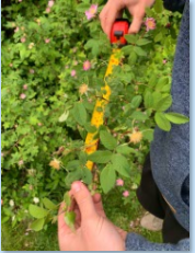
During the field data collection (including on June 13, 20, 27 and July 4) sunflower plants H1, H2, and H3 were observed to be the smallest (both in shoot height and maximum basal diameter) of the plants grown in the high-water volume study group (note: sunflower plants H1, H2 and H3 were all grown/ located within the same pot). The exact reason for this pattern is unknown, however, it may be due to variation in the microsite and/ or microclimate at this specific plant-pot location. All of the other sunflower plant replicates that were grown in the high-water volume study group (H4-H12) were noted to be larger (both in shoot height and maximum basal diameter) than the sunflower plants grown in the low-water volume application study group (L1-L12).
Blog Post 6: Data Collection
The hypothesis for my research project is the length of time an American Robin (Turdus migratorius) spends foraging in the meadow will differ from in the dog park. For my field data collection, I used the Pont Count method to monitor the length of time at least one Robin spent foraging in the meadow and the dog park. Ten replicates were carried out over ten days. For each replicate, I visited the meadow and dog park for 30 minutes each while alternating each day which location was visited first, and the field visits were conducted during the hours of 5:00-7:00 PM. The data collection strategy was relatively simple. Sitting quietly at a picnic bench with binoculars and a stopwatch, I recorded the time when at least one Robin present or absent in the meadow or dog park.
Considering the time of day, I was surprised by the number of Robins actively foraging and how easily they would return to each location once the area was vacant of dogs. It was also interesting to observe the behaviour between the Robins as one Robin appeared to be territorial over one particular tree and would chase any other Robins that would come near. Ultimately, it was interesting to see that the time a Robin spent foraging in the dog park was relatively close to the time spent foraging in the meadow.
Blog Post 6: Data Collection
Data collection at Mission Creek Regional Park is ongoing. Sample collection has been more efficient since reducing plot size to 100m^2. An additional area was selected to study approximately 500m east from the original site to increase the data pool, though this site has thicker brush which will make sampling challenging. To date, one of two study areas has been sampled (12 quadrats). Soil sample sites in each zone (riparian, floodplain, uplands) were selected, any further sampling is awaiting completion of a percolation test apparatus.
While it was initially observed Pinus ponderosa concentration was fairly constant through the gradient, it was since noted the tree characters change significantly. These observations have caused me to reflect upon my original hypothesis, warranting further investigation into stand make-up and quality, versus only tree concentration.
Blog Post 6: Data Collection
Hypothesis: Soil moisture affects presence and quantity of bracket fungi on mixed species trees in the Oxbow Trail Park.
Due to flooding that submerged large sections of my original study site, I elected to find a new site to complete my project. The area I chose is the Oxbow Trail park on Vale Island in Hay River, Northwest Territories. This park is comprised of wild mixed wood forest and creeks that drain to the Great Slave Lake and adjacent Hay River. It is largely untouched and sees very little foot traffic. For this reason, it is a good place to spot wildlife, including lynx, black bears and beavers. The other great thing about my new site is that unlike the first location, it is teaming with fungi. While I had a challenging time locating enough replicates at my original study site along the Kiwanis Trail, I quickly realized this would not be a problem in the Oxbow park.
For my initial study site I planned to run multiple transects and find the nearest polypore-infected tree for each transect. This strategy was chosen since the polypore-infected trees were quite rare, occurring only every 50-100 trees.
Since the presence of polypore-infected trees is plentiful at the Oxbow site, I decided to revise my strategy to incorporate stratified random sampling using randomly placed plots. I chose the stratified random technique because there were three distinct areas that I wanted to include: 1) The creek bed, 2) the forested area north of the creek and 3) the swampy forest south of the creek. I found plot coordinates using a random number generator. I sampled a total of 24 replicates, 4 from the creek bed, 10 from the north forest and 10 from the swampy south forest. This stratified breakdown gave a more accurate representation of the overall spatial context and distribution of trees. 16 of the replicates had polypores on them and 8 did not. I chose to study soil moisture content for trees without polypores to have a more complete understanding of the soil moisture distribution throughout the area.
Initially I only planned to count the number of brackets on each replicate and then take a soil sample from the base of the tree. However, during my field collection activities I felt it was also important to record additional details such as whether the tree was deciduous or coniferous, if the tree was alive or not, and if it was clustered amongst other infected trees. These additional findings may add more context to the study, however for the time being I am focusing only on the variables of # of fungi brackets and soil moisture content. I quickly discovered that many trees had brackets that extended far higher than I was able to count. Therefore, I only counted brackets up to diameter at breast height (DBH = 1.3) and then noted if multiple brackets were observed above this.
I initially planned on obtaining soil samples that were 20cm deep, however I found getting to this depth to be challenging due to roots, organic litter and the size of my spade. I therefore adapted my strategy and obtained all samples at a depth of 15cm, and tried to obtain approximately 100g of soil from each replicate.
To obtain soil weight and moisture content, I dried all the samples at 400 Celsius for 2 hours. Prior to drying, I weighed all the samples in the baggies that I collected them in, accounting for the weight of the bag. Once weighed, I placed the samples in the oven in batches. A few samples needed slightly longer to dry as they were very saturated. I considered the soil samples sufficiently dry when they crumbled easily, and no moisture could be felt. I reweighed the dry samples, accounting for the weight of the bowl, and then calculated the moisture weight and the soil moisture content percentage.
Now that my samples have been collected and calculations are complete, the next stage will be graphing the data and looking for any patterns or trends which will either support or reject my initial hypothesis.
Post 6: Data Collection
Last week I went out to collect the data for my field project. Low tide was particularly low – between 0 and 0.5m – and I had three days without rain. On Tuesday I did site a, on Wednesday site b, and on Friday I did sites c and d. At each site I did 10 replicates. It took me 10-20 minutes to generate, diagram & plan movement between the 10 co-ordinates, and sampling took between 19-58 minutes at each site (varying depending on how many oysters I was finding: site d only took 19 minutes, but 6 of the 10 samples had no oysters).
The sampling design worked fairly well. Once I placed the 1m x 1m markers, I looked for oysters, and for each oyster I added a tally mark to the “T” (for total) column, and then tallies for its position relative to the rocks. After collecting data at site b, I made the table where I recorded the tallies larger, because a couple of samples at site b had so many oysters that the tally marks didn’t fit entirely in one box. I also made a note to clarify that the “N” column, for oysters not in any rock shadow, includes oysters that are on top of or attached to the front of rocks. Oysters that are on top of a rock, but in the shadow of some part of the rock, are not included in the N column but in the relevant L, R, or B columns.
I think I may have to exclude sample 8 at site c, because that sample had 2 large rocks that were absolutely covered in oysters, to the point that that sample had 50 more oysters than any other sample. Because the rocks were covered, many oysters were behind other oysters, not behind any rocks. I recorded the ones behind other oysters in the “B” column because they are in the shadow of something breaking the wave action, but in hindsight I have no way of knowing which oysters came first, so some of the ones that are currently behind oysters may have not been earlier in their growth. For these reasons I think sample 8 can be disregarded.
Interestingly, an ancillary pattern seems to be that the difference between B and N is not large, but there are many fewer oysters found left or right than are found behind or not in shadow. I wonder if there might be something advantageous to the oysters to being towards wave action that only kicks in if the oyster is fully exposed – this might explain why there are many oysters behind rocks and not at all protected by rocks, but not slightly protected on either side. Or maybe there’s some aspect of fluid dynamics that means the water movement at the sides of rocks is worse than not near rocks.
Post 6: Data Collection
My data collection went quite well. Soil moisture can be affected by rainfall so I had to make sure I completed my data collection at one time. I collected my data on May 28th at around 1pm PST. It was a cloudy day, but it had rained quite a bit the day prior. I used pre-measured string to establish three transects about 10 m apart from each. One was along the top of the upper-slope, one in the middle, and one along the creek at the bottom. I placed five 16m2 quadrats on each transect, 4 meters apart from each other. This gave me a total of 15 replicates.
The biggest struggle I encountered was that the rain from the previous day had made the slope quite muddy and slippery. This made it especially difficult for me to place my quadrats and transect in the middle of the slope. I slipped a few times and got mud all over me. Another small difficulty was the insertion of the soil moisture meter. At some quadrats, I really had to push hard to get the meter all the way into the soil to the marker.
A pattern I noticed was that the soil moisture was around the same at both the top and bottom of the slope. However, the number of ferns was a lot more abundant at the top than at the bottom. This does not align with my hypothesis and I will have to reflect on some other factors on why this could be while writing my paper. I will take into consideration the greater shade at the top, as well as the bottom of the slope not being drained enough for ferns to grow.
Percy Herbert, Blog Post 6: Data Collection
I was able to collect measurements on 50 replicates at the Queen Elizabeth duck pond. 50 individual wild rose plants (Rosa acicularis) were observed. Ten replicates were recorded in each of the five height categories (1-50cm, 51-100cm, 101-150cm, 151-200cm, and 201-250cm). The heights of the plants were recorded as well as the distance from the apical bud to each of the first 15 vegetative buds.
Measurements were much more difficult to collect this time compared to the first data collection as the vegetative buds have all sprouted into small branches containing leaves and flowers. The new growth is all a vibrant green colour while the original stems are a rich red colour so it is still easy to tell the difference between the new growth and the stem. The new growth made seeing the measuring tape and the junctions of the new growth and the stem much harder. Although the measurements were harder to collect, with added time accurate measurements were still possible.
One issue with data collection is that for some of the shorter plants observed there were less than 15 buds. This is especially true for the 1-50cm category. This may lead to the exclusion of this category in some of the data analysis steps.
Initial data analysis appears to support the hypothesis. The spacing between the buds does not seem to be altered by plant height. An ANOVA will have to be conducted to confirm this observation.
Blog Post 6: Data Collection
I collected 61 replicates over the three stratified zones. Points were randomly generated using the “Random Points in Polygon” feature in QGIS. First, I determined the area of each of my zones using QGIS. They were as follows:
Alder Zone (zone 1): 7895m2
Grand fir/ Douglas-fir Zone (zone 2): 24239m2
Arbutus/ Garry oak Zone (zone 3): 10932m2
Based on the proportion of the total area that each zone represented, I divided up the 60 replicates to attain the following sampling intensity:
Zone 1: 12 (rounded up from 11.5)
Zone 2: 34
Zone 3: 15
I exported the random points as a GPX file and loaded them onto my GPS. In practice, the sampling strategy worked fairly well. It was difficult to reach some areas due to shrubby undergrowth, but since the areas which were dominated by shrubs lacked H. helix, I was able to visually assess these quadrats. A number of my points landed directly on the trunks of trees, and one landed on a well worn path. For these points, I shifted the sampling over by 2m to the north.
I noticed in my sampling that zone 3 is not entirely contiguous, with some small patches of Douglas-fir dominant stands. Overall, only two points landed in one of these patches, and these data points were not dissimilar from other replicates in the same zone. Since Douglas-fir is able to cope with some level of water stress, I don’t think this is compelling evidence against my stratification. Visually and by touch, the soil is drier in this area, regardless of the presence of arbutus and garry oak.
Reudink, Post 6: Data Collection
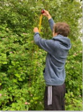
To collect my field data, I established three transects through the 0.68 ha forest area under investigation and systematically placed six circle plots with a 5m radius 20 paces apart in each transect. Altogether there were 18 replicates. I am interested in the density of large Populus alba trees and the associated soil moisture, so at each circle plot I extracted a soil sample at the centre of the plot and measured the circumference of each large tree at breast height (above 25cm in circumference). I made sure to dig at least 10cm deep when collecting soil samples and removed any gross organic material before taking any measurements. My sampling design went quite smoothly; however, there was a recent snowstorm that covered my study area in snow, so walking and digging was more time consuming and I also had to be careful when extracting soil samples to not contaminate them with the surrounding snow. Once I got back to my house, I sorted through the soil samples to make sure there was no organic matter and then weighed them all, put them in the dehydrator at 115˚ F, then weighed them again. I used the resulting value to calculate the soil moisture content percentage.
While walking through the dense forest and seeing my data unfold before my eyes, I noticed that the centre transect was having a greater density of P. alba then my east transect. This was surprising to me because I initially believed that my peripheral transects were both denser in P. alba than the centre transect. When reflecting back to my current hypothesis (P. alba density is associated with soil moisture), this reaffirmed my suspicion that increasing soil moisture content was going to be associated with increasing P. alba density. This is because the tree density was increasing from east to west and there was a dyke near the west perimeter, so I assumed that soil moisture would similarly be increasing in a westward fashion.