Blog Post 6: Data Collection

To date I have gone out twice to collect field data at my grasslands site in Vernon BC. To this point I have sampled ten replicates. Each replicate is a different transect line along a slope gradient from a gentle lower slope position to a steep mid to upper slope position. On each replicate I have sampled 4 plots, totalling 40 plots. I have not had any particular difficulties implementing my sampling design.

A point of observation that I made on September 26th, on my second data collection day was that soil samples on the lower slopes demonstrated hydrophobic reactions to the water I added in conducting the texture analysis. I did not notice this pattern with the soil on the steeper slope position. This will be a point of further research into soil property characteristics.

I have not noticed ancillary patterns, however I have noticed that the vegetation has a quite a distinct zonation between gentle and steep slope sections, with predominately grasses on the gentle slope and forbs/shrubs on the steep slope section.

Blog Post 8: Tables and Graphs

Given that I am working with data from 10 transects with 11 quadrats each, I had a great deal of trouble organizing my data.  I took field notes in a Google Sheet and used Excel for calculations and data analysis from home.  There were a total of 25 forb species found in the study area and I collected moisture, cover and species abundance data; therefore, (including empty sets) I have 2750 data points (10 x 11 x 25).  It became clear very quickly that naming convention was extremely important when trying to arrange and analyze my data in a meaningful way.  For example: I initially designated my quadrats as T1Q1, T1Q2… T10Q11 (with the number succeeding the “T” being the transect number and the number succeeding the “Q” being the quadrat number).  However, when sorting data alphabetically, T10Q11 would be arranged between T1Q11 and T2Q1.  Therefore, I had to go back and change my naming convention to T01Q01, T01Q2 etc.  This seems like a simple thing, but it caused me a great deal of trouble and illustrated the importance of having “data management-friendly” naming conventions.  I will note that this is, certainly, not the only time I needed to go through and “clean” my data in order to facilitated organizing it in a logical way.

Concerning presenting my data: I struggled to find a singular figure that would readily summarize the overall trends in my project without being convoluted or confusing.  Therefore, I decided to submit a singular graph of the the Shannon-Wiener Index against distance (from the shoreline of the South Saskatchewan River).  I will also note that I did perform calculations for Simpson’s diversity index but have only included the Shannon-Wiener in my submission to avoid ambiguity.

I expected that forb species diversity would be highest at an intermediate area between the extreme ends (the shoreline and the uplands) of the riparian environment I was studying.  While this is true (Figure 1), I was not expecting that the highest level of diversity would occur that close to the shore.  In addition, I was not expecting that forb diversity would be so high approaching the uplands.  While not pictured in this graph (again, for the purpose of keeping it understandable), soil moisture steadily declines and elevation increases as distance increases.  But soil moisture, alone, does not account for the low diversity found from 25-50 m.  Fortunately, I’ve also collected data regarding shrub cover (that I suspect limits forb species).  I also have elevation data from each quadrat and am thinking about using it to calculate the steepness of slope gradient.  As I was sampling my transects, I noticed that both of these factors seemed to relate to quadrats in which no forb species were found.

Regardless, I still have some statistical analyses to perform in order to know which results are significant.

Blog post 2: Sources of scientific information

Trophic ecology of alpine stream invertebrates: current status and future research needs.


This article on ecology is an academic peer reviewed review. The article is written as part of a doctoral dissertation in affiliation with a university (Fureder and Niedrist 2017); these authors can be considered as experts in the field.  It contains citations throughout and a bibliography at the end, this and the expertise of the authors makes this an academic resource. There is an acknowledgement to two anonymous referees making it a peer reviewed paper.  Finally, it would be considered a review as there is no methods or results section.


https://eds-b-ebscohost-com.ezproxy.tru.ca/eds/delivery?sid=45b0b78a-8552-49f4-9830-4bd75c899487%40pdc-v-sessmgr02&vid=10&ReturnUrl=https%3a%2f%2feds.b.ebscohost.com%2feds%2fdetail%2fdetail%3fvid%3d9%26sid%3d45b0b78a-8552-49f4-9830-4bd75c899487%2540pdc-v-sessmgr02%26bdata%3dJnNpdGU9ZWRzLWxpdmUmc2NvcGU9c2l0ZQ%253d%253d


Fureder L, and Niedrist G. 2017. Trophic ecology of alpine stream invertebrates: current status and future research needs. Freshwater Sci. 36(3): 466-478. Doi:10.1086/692831

Blog Post 7 Theoretical Perspectives

My research is primarily concerned with the presence or absence of conks growing on trees. This relates to tree health, possibly opportunistic pathogens, and succession of a second-growth forest.

An idea that underpins my research is conk prevalence in one area of Mundy Forest. Is it a natural environmental condition, is it there because of tree disease and is the tree decaying before the presence of conks or because of it? It also touches on disturbance regimes and the successional stages of the forest (micro-disturbance from the death of trees allowing more lower canopy growth with additional light availability). The typical forest structure of the Pacific North West includes an iconic species, Western redcedar, in which climate change is strongly affecting the typical forest diversity. Changes in precipitation, temperature and drought patterns are affecting the distribution and health of Western redcedar. This may be an idea underpinning my research of tree health or decline and may have nothing to do with conks.


Tree health, opportunistic pathogens, climate change, bracket fungi

Observations 1

07/09/2020

08:47

8 °C overcast

-transition season with summer ending and moving into fall, rainfall in the past 24hours


The site is located on Steamboat Mountain and is designated as rangeland, specifically the Bryanton Creek and Tea Kettle ranges.  It is a mountain slope with primarily conifer forests. I chose three small perennial streams that flow through the area (Figure 1). Each of the sites shows recent use by cattle (Bos Taurus) with tracks and manure.  The slope to access the creeks at the point of observation is varied for each location; site 1 location 4 is forested and has little slope (Figure 2), site 2 location 2 is steep, rocky and has small areas of pooling (Figure 3), site 3 location 3 is gently slopped with steeper sides (Figure 4). The streams are rocky and varying sizes of pooling with gravel to muddy linings.  All three sites have similar vegetation with large spruce (Picea ?), birch (Betula papyrifera),and Douglas fir (Pseudotsuga menziesii var. glauca) forming the primary canopy.  There is an abundance of red-oiser dogwood (Cornus stolonifera C. sericea), common horsetail (Equisetum arvense), and bunch berry (Cornus canadensis) as well as mosses and lichens at all three sites.

Figure 1 Creek locations created on iMapBC
Figure 2 Creek site 1
Figure 3 Creek site 2
Figure 4 Creek site 3
Field notes

Questions that I had after observing these sites includes:


Is the health of the streams impacted by the cattle?

Is there concern with E. coli in the streams with the cattle defecating in the streams?

Does the access to the stream, as far as steepness, have an impact on how used the stream is by larger animals such as cattle and ungulates?

Blog post #5: Design Reflections

My initial sampling day went as planned insofar as I was able to collect data using the method of walking a transect and placing my quadrat after a random number of paces. I was even able to find my target species in some of the quadrats and record useful data. My sampling plan was flawed, however, as it assumed a higher density of dog strangling vine. I ended up covering the whole length of my study area before I was able to obtain 5 quadrats containing the target species. The issue is that, while abundant, the vine grows in a small number of patches. My initial design attempted to avoid sampling more than once from each patch by having a minimum number of paces, but this turned out to be a problem as there are only 4 patches in the particular treatment area I was sampling. Further investigation revealed the same issue in the other treatment areas. My study area doesn’t have enough Dog Strangling vine patches to be sampled in this way.

The response variable data collected was generally as expected. The number of seed pods on the plants reflected the different treatment areas as predicted in my hypothesis. The soil moisture or predictor variable measurements were not as expected. All of the soil was measured to be dry, regardless of the treatment area. During the sampling it became apparent that this was another flaw in the study design. To demonstrate that the slope or manicured areas had less water than the area along the creek (which seems to be the case based on the compaction and visual dryness of the soil), I would need data throughout the growing season that showed the plants consistently had less water. A simple snapshot would not demonstrate this effectively.

I am going to modify my sampling approach in two ways.

First, since my sample unit is the individual plant, I am going to sample the various patches in greater depth instead of using random paces and quadrats along a transect. This will provide several replicate areas within each treatment and allow for a larger number of individuals to be counted. A quadrat will be used within each patch to collect 3 or 4 separate samples, several meters apart from each other. A random number generator will be used to determine random locations within each patch for sampling.

Second, since I can’t demonstrate that water availability is different across time between the different treatment areas. I will have to rethink my hypothesis. The data supports the observation that there is a gradient in the number of seeds between the different treatment areas so the predictor variable will be modified to be the different treatment areas themselves within the study area.

These two modifications will allow for significantly more individuals to be sampled within the study area while maintaining random selection, and allow for a hypothesis that is verifiable or refutable.


Blog Post 6 Data Collection

I collected my field data on 2 separate days (March 4, 2020, and August 6, 2020). The second survey day was to address my initial field survey design flaws. I needed to replace my dropped eastern auxiliary plot (as the original had been in Lost Lake) and to collect 5 more replicates. I increased the number of replicates, as 10 is the oft-repeated rule of thumb for a variable of interest.

As I now have 10 replicates, and 4 trees surveyed at each replicate, I have 40 trees sampled. I used the Vegetation Resources Inventory (VRI) Ground Sampling Procedures methodology to replace my dropped auxiliary plot. I also used these methods for 5 additional replicates, totalling 10.

August 6th was overcast, 20 degrees Celsius and called for rain. It had rained in the morning and I had hoped to collect data within the opening that rained ceased in the afternoon. I was unlucky and I had also not made my data sheets on water-proof paper. It was really difficult and an oversight I would never do again.

In my hypothesis, I stated that I would find conks on only one tree species and that is currently not being supported by my data. I have found conks on deciduous and coniferous trees. What is being supported is that conks appear on trees that have some type of decline present.

Blog post #4: Sampling Strategies

The three techniques I used were: systematic area, random area and haphazard.

The fastest method was systematic area with a total time of 12 hours, 37 minutes. Second fastest was Haphazard with a total time of 12 hours, 56 minutes. The longest sampling time was random area with a total sampling time of 13 hours, 14 minutes.

The calculated percent error for the most common species:

Eastern Hemlock

systematic area: 1.25%

random area: 22.58%

haphazard: 2.14%

Sweet Birch

systematic area: 8.94%

random area: 94.04%

haphazard: 21.7%

The calculated percent error for the least common species:

White Pine

systematic area: 4.76%

random area: 42.86%

haphazard: 52.38%

Striped Maple

systematic area: 100.00%

random area: 128.57%

haphazard: 14.28%

The accuracy was better with the higher density species. As the density lowers, a much higher error occurs. Using a systematic area method had the best chance of a low error with errors generally below 10% except where the species was not detected at all. Haphazard also produced lower errors while the random area method produced errors of at least 22.58% ranging up to 128.57%.

Blog Post 7: Theoretical Perspectives

My hypothesis (that the community structure of forb species changes as elevation increases within a riparian environment) is likely related to several underlying processes within my study area (located on the Eastern bank of the South Saskatchewan River in Saskatoon). The underlying processes that (appear to) impact the types of forbs and their abundance along the elevation gradient are soil moisture/type, cover, competition, and disturbance.


I have soil-sampled (through hand texturing) each of my quadrats and it seems that the soil moisture content is related to the types of forbs that I find at various elevations. I initially expected to see a steady decline in soil moisture as elevation increased; however, soil moisture was not directly related to elevation in all locations. Areas with dense shrub cover appear to have higher soil moisture than areas without cover at similar elevations. In addition, the quadrats shaded by heavy shrub cover do not appear to have the same community structure as quadrats with similar soil moisture and are not shaded. Therefore, this has led me to believe that competition from shrubs and canopy cover may also influence the community structure of forbs in the area.


Finally, it is notable that some transects have an elevation difference of 25 meters (from the lowest quadrat to the highest quadrat). The study area maintains a (relatively) consistent river depth throughout the year because of its close proximity of a weir (which was constructed for the purpose of maintaining a consistent water level within the city). Therefore, flood disturbance does not likely play a major part in community structure at higher elevations. However, the modest fluctuations in river depth do submerge the lowest quadrats when the river is high. Therefore, flooding may also be an influence on forb community structure within my study location.


On a broader, theoretical level: different species of forb within my study area are likely to have a wide variety of adaptations to deal with disturbance, water submergence, drought, and shade. While these adaptations remain unknown to me at the moment, I can speculate on several adaptations that some of the forb species may have. For example: it is possible that drought tolerant species (found closer to the uplands) have deeper roots (that can penetrate lower in the soil to access groundwater) than the forb species that exhibit a preference for areas with higher levels of water saturation. Conversely, species that exhibit a high preference for low elevations may have adaptations to prevent them from becoming waterlogged by high levels of water saturation.


Keywords: Riparian vegetation, forb community structure, elevation gradient

Blog Post #3: Ongoing field observations

The organism that I plan to study is Vincetoxicum nigrum or Dog Strangling Vine. More specifically, the seed production of the vine.

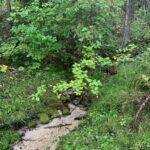
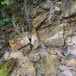
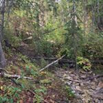
Along the north/south length of my study area, I can find the vine growing in the densely vegetated area between the creek and the pathway on the west side of the study area as well as along the hill side, on the east side of the study area. I do not see it growing in any substantial way in the manicured grass area between the slope and the pathway, however it is possible that the vine is trying to grow there but is impacted by the grass cutting.

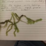
I have noticed that the vines in the densely vegetated area appear to be healthier and more productive than the vines growing along the slope. In the vegetation the leaves are stiff and the vines are tall, wrapping around many other plants and spreading out. On the slope, the leaves are wilted and soft. The vines do not grow as tall on the slope either. Event where a tree or bush provides a possible climbing aid.

A few things may be causing this difference in plant health. Perhaps the amount of sunlight on the slope is too high. Or maybe there is more nutrient available in the wooded area. During site observations, I noticed that the soil on the slope is very hard and dry whereas the soil in the wooded area is noticeably wetter. This is consistent along the north/south length of the study area. It is a common sight in the surrounding area to see large patches of Dog Strangling Vine growing in full sun, on slopes. The difference is probably not too much sunlight. I suspect that reduced water availability would impact the plants ability to perform transpiration, which as a result, would impact the level of nutrients brought into the plant, with the water, for growth and reproduction.

Considering the above, I hypothesize that differences in water availability are impacting the vines ability to grow and thrive. My prediction is that plants in drier soil will produce fewer seed pods.

Based on my hypothesis and prediction. The predictor variable is soil moisture and the response variable is the number of seed pods per plant. The number of seed pods would be counted on a numerical scale and so would be a continuous variable. Depending on the measurement device, soil moisture could be categorical – in the case where a moisture probe simply displays one of a discrete set of value: dry, moist, wet, etc..) or continuous  – in the case where a moisture probe displays a spectrum of out puts ranging on a scale from dry to wet. In this case, the moisture probe in use displays a spectrum and so would be considered continuous.

notes August 16 notes August 23 Photos August 16-23