The observation site (The Site) is located at King Street East and Bond Street on the Harmony Creek trail in Oshawa, Ontario. The site is located in an urbanized park with an engineered flood plain and built habitat. The site extends approximately 40 – 50 metres from the harmony creek (which runs north south along the west boundary of the site) on the west to the guard rail of Bond Street on the east. The site follows the creek for approximately 80 metres from a tunnel where Harmony creek passes below King Street in the south to a park bench at the north boundary.
The east creek bank is vegetated with trees, flowering plants and small shrubs. These plants, trees, and shrubs extend from the creek bank, approximately 5 metres to the Harmony Creek Trail – which is paved with asphalt. On the opposite side of the trail (east side), the flood plain is vegetated with manicured grass for approximately 15 – 20 metres. To the east of this grass is a slope that forms the upper boundary of the flood plain. This slope is vegetated with tall grasses, flowering plants and several mature trees.
Time: 4:15 pm. August 9, 2020. Mid-late summer.
Weather:
Partially cloudy. Winds 20 km SSW. 27 degrees Celsius.
Observations:
A construction site is set up to the south of the observation area. The path under King street is closed with fencing.
Crickets audible in the vegetation near the creek at the south end.
Grass is dry and brown to the east of the path.
House sparrow observed on the path. It is flying back and forth between from shrubs and the asphalt. Shrubs have grape vines in them.
Creek is running calm and clear. No fish observed. No odours or sheens observed. The construction team has installed some netting in the creek.
Grassy area on the slope to the east has Dog Strangling Vine growing on it. Vine looks de hydrated. Leaves are shriveled.
Monarch butterfly observed flying through the area. No milkweed observed during inspection.
Questions:
What avian species frequent the area?
Is the dog strangling vine spreading? The vines looked to be stressed. Are they producing seeds?
The creek runs through an urbanized area with significant human impact, are any fish species present? Are there any species that run upstream to spawn in the fall at this location?
I have been collecting data for eight weeks over the course of the summer, to coincide with the mating season of frogs and toads on Prince Edward Island. I had four replicates at five locations randomly chosen throughout the South Shore Watershed of Prince Edward Island.
Every two weeks, I would visit five sites after sunset and record their mating calls with my iphone and I also recorded any visual sightings. Prior to the start of my data collection, I placed water temperature loggers at each site, so I was able to record water temperature for each night I was recording the calls. I did not have any trouble sampling, with the exception of mosquitos that attacked me mercilessly. I haven’t noticed any patterns that necessarily agree or disagree with my hypothesis-It is difficult to determine species abundance, especially at night with frogs. I am concerned that my data will show more correlation with mating season than farming. I have already figured on confounding factors based on their actual breeding patterns. I often find myself in these locations during the day, and I am able to see an abundance of leopard frogs, but I don’t hear them at night when recording. Conversely, I never see Spring Peepers, but I record them in abundance.
I have decided to do an abundance study of frogs and toads of PEI and their distance from active farming sites. We only have four frogs-some will say five, but the pickerel frog hasn’t been seen here since 2003, and one toad. The green frog (Rana clamitans), the wood frog (Rana sylvatica), the leopard frog (Rana pipiens), spring peepers (Pseudacris crucifer), and the American toad (Bufo americanus).
My hypothesis is that the species abundance increases as the distance from active farming increases.
I have chosen five sites at random, however, I had to make sure that they had the right environment to support the frogs and toads, so they are all fresh-water riparian sites. I chose those sites and will be measuring the distance to active farming sites through arcGIS. I had some water chemistry analyzed at each of the five sites, however, I only had the funds for one sample at each site, so, depending on their nitrate and phosphorous levels, I will maybe only use this data in my discussion, to hopefully support my hypotheses.
I will drive to each of the five sites during the breeding season at dusk and record their calls for five minutes with my iPhone, then analyze the recordings using their call to identify them and the Abundance Code for Frogs to determine how many are calling:
0 = no amphibians heard
1 = individuals can be counted (no overlapping calls) – estimate of 1-5 individuals calling at site
2 = calls of individuals are distinguishable, but some calls overlap – estimate of 6-10 individuals calling at
site
3 = full chorus, or continuous calls, where individuals cannot be distinguished – estimate of more than
10 individuals calling at the site.
Frogs only call during mating season, so I intend to do 20 site visits (4 nights, at 5 sites) during this time.
Preamble: After reassessing my planned sampling methods and study site, I began collecting my formal data on August 5th, 2020. In this blog post, I have included information regarding some changes to my project. I have opted to include these updates in this post, rather that the original blog posts to avoid the need for the reader to navigate to my other blog posts to understand the context in which this data was collected.
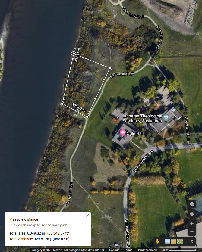
Study site updates: Due to the difficulty in navigating some of the steep slopes within my initial study area, and avoiding some areas that may confound the project, I have redefined my study site. The original study site was an area of approximately 38 576 m2 in size and encompassed a ravine. I desired to study the forb species abundance and distribution along the riparian-upland gradient on the eastern bank of the South Saskatchewan River. However, the ravine threatened to confound my project (having a separate species profile and elevation gradient), and some of the cliffs within the original study area were going to be too difficult to navigate. Therefore, the study area was reduced to 6 349 m2 and is depicted in Figure 1.
Hypothesis updates: My original hypothesis involved investigating forb species abundance and distribution as they relate to the distance from the river. However, I have now opted to shift my focus towards elevation (rather than distance). Furthermore, in an attempt to address the processes behind forb abundance and distribution, I have decided to estimate soil moisture along the gradient.
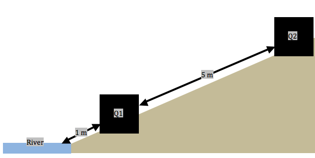
Sampling method updates: Following some advice and reflection on my proposed sampling methods, I have decided to adopt a systematic sampling approach (along transects) within the study area. Each transect will run perpendicular to the shore of the river and contain 11, 1 m2 quadrats that are spaced 5 meters apart (Figure 2). Ten randomly generated locations at the shore of the river were chosen and the first quadrat in each transect is to be laid at 1 meter from the river’s shore. Along these transects: I have been collecting forb species abundance, noting the proximity to river, estimating soil moisture (by hand texturing), and noting whether there is a tree/shrub canopy hanging over the quadrats.
Data Collection: Three replicates (transects) were sampled on August 5, 2020 between 9:30 AM and 6:30 PM. As stated above, each transect consisted of 11 sub-samples (quadrats).
Transects proved difficult to implement because the slope was extremely steep in some locations. Working from the river, I would lay a quadrat, collect data, then measure 5 meters to the next quadrat location. Some locations arose where I would not be able to move in a straight line (often up a cliff); therefore, I would have to mark the location of the previous quadrat, navigate to the new location via an alternate route, and measure backwards to maintain a consistent distance between quadrats. In addition, the upper area of the riparian zone is dominated by dense stands of Caraganasp. and Amelanchier alnifolia (Saskatoon berry) shrubs. This region was particularly time consuming to navigate; however, it was still feasible. The locations with a dense shrub canopy exhibited a notable absence of forbs. Therefore, at the sixth quadrat in transect one, I decided to begin noting when a canopy of shrubs or trees hangs over each quadrat. In order to maintain consistency, I navigated back to the previous five quadrats to collect this data before continuing to the seventh quadrat in the first transect. Overall, the largest problem in implementing my sampling technique was time. Not being able to complete all ten of my replicates in one day will mean that I may not have consistency with soil moisture between sampling days. This can be mitigated by ensuring that my sampling is, in the very least, completed within a timely manner (over the next few days). In addition, I will be navigating to some of my previous points on subsequent sampling days to verify that the moisture content of the soil has not changed. If it has, I will need disregard my previous soil moisture data and plan for an individual day of soil sampling to control for moisture variances.
Despite having only sampled from three transects, I am noticing ancillary patterns related to my hypothesis. The transects closest to the river are all saturated with water and this saturation level quickly declines as you move up in elevation. Consequently, many forb species exhibit preferences for different elevations. For example, Astragalus pectinatus (narrow-leafed milk-vetch), Cirsium arvense (Canada thistle), and Liatris punctata (dotted blazing star) display an extreme preference for dry (0-25% saturation), upland locations. In addition, Hedysarium alpinium (alpine hedysarium) and Astragalus americanus (American milk-vetch) are strongly associated with heavily saturated (75-100% saturation), low elevations. However, some forb species like Solidago canadensis (Canada goldenrod) do not appear to display a preference for any elevation or moisture content.
Figure 1: The figure above is an image taken from Google Maps depicting the redefined study area.
Figure 2: The figure above is a diagram depicting the location of the first two (Q1 and Q2) quadrats in a transect. Q1 is positioned 1 m from the river and every subsequent quadrat is placed 5 meters away from the previous quadrat, along a perpendicular line extending from the edge of the river.
REFERENCE LIST:
Google Maps [Internet]. c2020. Canada: Google Maps; [accessed 2020 July 29]. https://www.google.ca/maps/@52.1378074,-106.6412387,549m/data=!3m1!1e3
I used the area based systematic, area based random, and area based haphazard methods to sample the Snyder-Middlesworth Natural Area.
The area based haphazard method had the fastest sampling time at 12 hours and 28 minutes, followed by area based systematic at 12 hours and 46 minutes, and area based random at 12 hours and 52 minutes.
Percentage error for the two most common species:
Eastern Hemlock
Systematic: 8.1%
Random: 5.1%
Haphazard: 1.6
Red Maple
Systematic: 5.8%
Random: 29.7%
Haphazard: 22.6%
Percentage error for the two rarest species:
Striped Maple
Systematic: 100%
Random: 28.6%
Haphazard: 18.9%
White Pine
Systematic: 90%
Random: 48.8%
Haphazard: 98.8
There appears to be a strong correlation between higher species abundance and higher sampling accuracy, with significantly higher percentage error in the sampling of the rarest species than the sampling of the most common species.
For the two most common species i found the systematic sampling strategy to be the most accurate, while for the two rarest species Random sampling was the most accurate. There appeared to be great variation in the accuracy of the three strategies, and there was no overwhelming stand out in terms of accuracy.
I used systematic sampling across each of my three cross-sections to study soil moisture, using a 7inch probe, along the slope of my chosen area. At each interval I’d measure one soil moisture reading, the percent slope using a level and ruler, and the presence/absence of trees in a 2m2 radius.
There were a number of key issues I ran into throughout this process. The process of systematically sampling horizontally across the slope and taking only one reading at each stop did not always render replicates with similar slopes for comparison. In order to address this issue moving forward, I may have to modify my design to include taking more than one percent slope and soil moisture reading within each quadrant to ensure replicates and/or set pre-determined ranges for what constitutes a mild, moderate and severe percent slope for clarity purposes. The second issue I ran into was using my equipment in a consistent manner. Initially I would insert the soil moisture probe to its maximum depth, but ran into issues in later sampling when this was not possible due to soil conditions. To ensure the accuracy of my results in future sampling, I need to improve the consistency from which depth I take my soil moisture readings. I can accomplish this by either taking moisture readings at various depths at each point or marking an insertion limit on the probe itself at some point <7inches to ensure that it’ll be consistently inserted to the same depth. Other general modifications to future sampling will include expanding the size of my quadrants to improve data collection regarding tree sampling, and to gather more detailed information regarding the observed trees in order to better understand the potential impact of soil moisture, as it pertains to slope, on their growth. I will continue to implement systematic sampling; however, it will obviously need to be adapted to account for the larger quadrant sizes. I will also look into whether there is a way to accurately, and more efficiently measure percent slope since using a level and ruler was a tedious, and time-consuming process that will only become more challenging with more sample points.
The results were surprising to me in that they were not aligned with my prediction. I predicted soil moisture would be highest at the bottom of the slope, and what I found during this preliminary research was that it was highest at the midpoint. I have some ideas about why this might be, but evidently, I will have to wait until I’ve collected more data to comment on the findings with any reliability.
In the virtual forest tutorial, I chose Mohn Mill as my community sample. I chose to do area-based sampling using haphazard, random, and systematic methods. The haphazard method of sampling had the fastest estimated sampling time at 14 hours and 48 minutes, followed by the systematic method (16 hours and 59 minutes), and the random method (18 hours and 13 minutes).
Percentage errors of the two most abundant species:
Red Maple:
Haphazard- 2.68%
Random- 8.20%
Systematic-11.5%
Chestnut Oak:
Haphazard-2.90%
Random-2.05%
Systematic-5.08%
Percentage errors of the two least abundant species:
White Pine:
Haphazard- 100%
Random- 54.4%
Systematic-53.9%
Downy Juneberry:
Haphazard-44.0%
Random- 53.9%
Systematic- 57.0%
It is clear from the data that the more abundant species were more accurate than the less abundant ones. Overall, the random method was most accurate, followed by systematic, and then haphazard. Although haphazard sampling is more time efficient, it is not as accurate as the other two methods. It surprised me to see that haphazard sampling was the most effective for common species and that random/systematic sampling was most effective for uncommon species. I would expect haphazard sampling to be more effective for less common species, as samples are chosen subjectively. I would expect systematic sampling to be most effective for common species. My surprising results are likely due to my not taking enough samples before collecting and analyzing the data or poor choices when choosing quadrants to sample.
The biological attribute that I plan to study for my field research project at Erlton/Roxboro Natural Area is soil moisture along a slope. The pattern that led me to this question was the distribution of trees across my gradient. The bottom of the slope was marked by a canopy of large trees, the middle of the slope consisted of frequent, medium-sized trees while the top of the slope was marked by infrequent, notably smaller trees and saplings. I plan to combine these two pieces of information to determine how the angle of the slope impacts soil moisture, and subsequently investigate whether this is a potential limiting factor for tree frequency, and size.
I will conduct my research over the entire area of my slope, but will subdivide it into three horizontal cross sections in order to capture three distinct percent slopes. The first will be just under the top of the ridge on the steepest part of the slope, another will be at the midpoint where it is more moderate and the last one will be at the bottom where the earth is essentially flat (see attached scan below).
I hypothesize that slope will impact soil moisture levels and I predict that soil moisture will be negatively correlated with percent slope and positively correlated with tree frequency and size. Furthermore, I predict that there will be a trade-off between tree frequency and size and that as soil moisture reaches it’s maximum, tree frequency will decrease while size increases.
Potential Response Variable: Soil moisture level (instrument specific – could be either)
I conducted area-based systematic, random and haphazard sampling methods on the Snyder-Middleswarth Natural Area in the virtual sampling tutorial. Eastern Hemlock (EH) and Sweet Birch (SB) were the most common species found in my simulation, while Striped Maple (SM) and White Pine (WP) were the rarest.
Systematic sampling was performed on 25 quadrats over an estimated duration of 12hrs37mins. The percent errors for EH, SB, SM and WP were 11.47%, 21.70%, 100% and 90.48%, respectively.
Random sampling was performed on 24 quadrats over an estimated duration of 12hrs57mins. The percent errors for EH, SB, SM, and WP were 29.39%, 17.02%, 90.29% and 100%, respectively.
Haphazard, or subjective, sampling was performed on 24 quadrats over an estimated duration of 12hrs40mins. The percent errors for EH, SB, SM and WP were 28.58%, 6.38%, 76% and 197.62%, respectively.
Estimated sampling times were comparable across all three methods; however, systematic sampling had the lowest time and included an additional quadrat, making it the most efficient strategy in this simulation. In terms of accuracy, the margin of error was consistently, and considerably, lower among common tree species (EH & SB) as compared to rare tree species (SM & WP). This finding suggests a decrease in sampling accuracy when dealing with rare tree species.
In this simulation, systematic sampling was the most accurate for two out of the four tree species (EH & WP) and the least accurate for the other two species (SB & SM). Random sampling was never the most accurate method of sampling but it was only the least accurate for EM, by a very small margin (0.81%). Finally, haphazard sampling was the most accurate strategy for two out of the four tree species (SB & SM) and the least accurate method for WP, by a substantial margin (97.62%).
While the results from this simulation are inconclusive, I submit that systematic sampling was the most accurate. It was at par with random sampling for rare tree species, but slightly outperformed it when sampling common tree species. Furthermore, while haphazard sampling yielded the lowest result among the findings (6.38% error for SB), this sampling technique generally yielded inconsistent results. Increasing sample size in future simulations would improve accuracy across all three sampling methods.
I have decided to study vegetation abundance with increasing distance from the creek.
Cows Parsnip (Heracleum umbellifers)
Sweet Clover (Melilotus officinalis)
tufted vetch (Vicia cracca)
White Clover (Trifolium repens)
grasses
I choose four spots along the creek to observe the plants growing there and noticed that wherever the Cows Parsnip was growing, no other plants (besides grass) were growing. The other wildflowers grew everywhere on top of the creek bank, but not near the water. The Cows Parsnip seemed to grow closer to the creek and in damper areas. They also grew more in the shade, while the other wildflowers appeared to grow where there was more sun.
Near Greenhouse.
The wildflowers only grew on the banks of the creeks. The banks here are very steep and the only organism growing near the water is grass. Wildflowers are covering the field next to the walking trail.
2. Near Library.
I stopped seeing the other wildflowers when the Cows Parsnip begins to show up. There is a group of approximately 20 of them in this area. They are in the tall, damp grass and under the shade of the tress. The banks are more shallow here so the other wildflowers are growing closer to the creek.
3. Kin Park Bridge.
The Cows Parsnip are flourishing on the shallow decline to the creek. They are about 2-3 meters from the water. The closer they get to the creek, the larger and more green they are. The other wildflowers stop near the top of the bank.
4. Across from baseball diamond.
There are tons of Cows Parsnip growing here. There are no other wildflowers here. The Parsnip appears to be greener and have whiter flowers closer to the creek.
It seems as if Cows Parnsip is better suited to survive harsher condition than the other wildflowers. They continue to thrive without sunshine and in very damp areas.
Hypothesis:
My hypothesis is that proximity to the creek will effect the variety of plant life growing in the area.
Prediction:
I predict that the Cows Parsnip will survive closer to the creek due to it being more resiliant to harsh conditions, whereas the vegetation that need more specific conditions (sunlight and water) to survive will not. I predict that the as distance from the creek increases, the variety of plantlife will also increase.
A possible response variable is the presence/absence of the types of vegetation (categorical) and a possible explanatory variable is their distance from the creek/shade of trees (continuous).