Blog Post 5: Design Reflections

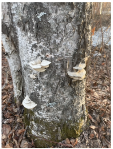
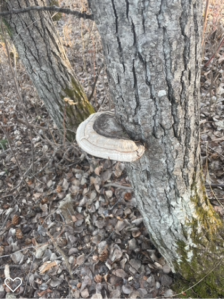
I had two main difficulties when establishing the sampling of my research area. The first issue was establishing quadrats of equal size due to the terrain. I initially wasn’t sure how I was going to measure out this distance given the uneven terrain and thick tree cover. However, I decided that using a string pre-measured at 20m worked better than trying to navigate through the forest with a tape measure. Using this method I did manage to space out several 400m2 quadrats and will create more to further my research. Using this method I found it easy to search for my response variable (presence of bracket fungi on trees) and will continue to with this method.

The second significantly bigger challenge that occurred was the annual spring break up of the river which flooded out a large section of my study area. I initially established my quadrats starting from the bridge and ending near the high school. However, about a 500m stretch of park was entirely flooded due to record-high water levels. I therefore had to adjust my study area slightly and anticipate being unable to establish quadrats in the flooded areas. This was a shame because I had visualized bracket fungi on a few of the trees in these now flooded areas but did not get a chance to study them before the water level rose. It is unlikely I will be able to access these areas again for the duration of the course.

For my sampling method I opted to use the quadrat method, using the Kiwanis trail as a makeshift transect. This allowed me to study areas on both sides of the trail, which vary a fair bit in terms of species abundance and moisture content. However, at present, most areas on the east side of the trail (closer to the river) are inaccessible, therefore for my initial study, I only included counts from quadrats on the west side of the trail which weren’t waterlogged. I suspect the water in the east areas will recede within the coming weeks so I may be able to resume sampling in these areas later. However, if the water level does not recede, then I will adjust my study method and create a transect west of the trail rather than studying quadrats on the east side that may continue to be inaccessible. The key downside of this modification to my research methods is that it cuts out the trees nearer the river that sit on a steeper slope and are subjected to different environmental conditions to those trees inland. I was hoping to see if any key differences could be found between trees based on their proximity to the river

On a final note, I am still struggling to determine what to study for the predictor variable(s) and how to go about measuring them.

Blog Post 8: Tables and Graphs

At this point, I have completed the collection of all my data. In the Small Assignment #5, I have made some graphs using the data I collected from the field (garden) for this experiment.

My graph demonstrates the relationship between the number of other types of plants growing in 30 cm from each bean plant (sample plant), and each individual plant’s growth estimated using its leaf and bean pod numbers. Each graph is a representation of sample data from one garden bed. While summarizing my data, I did not have any major difficulties, but it rather helped me to see if really there was a correlation between both the independent and dependent variables. It also helped me to eliminate one row of data recorded from when I collected data, in which all numbers were 0, except for only one sample, in which there were 6 flowers per bean plant.

Referring back to my hypothesis, which involved determining whether the presence of other plant species growing near an individual bean (Phaseolus vulgarus) plant contributes to its growth and abundance. When I did the experiment, I was looking forward to understanding whether greater diversity in garden plots would reduce the intraspecific competitions; therefore, leading to larger bean plants. However, the results obtained from the experiment, were unexpected, as I anticipated a positive relationship between the growth of the bean plant, and diversity of plants near it. Some of the results indicates a negative correlation, others weak positive correlation, and the rest show no correlation. This opened my mind to further explore the effect of greater diversity of plants in the same garden bed, or in a close area. I also want to explore the effects of interspecific as well as intraspecific competition. I wonder if either ever favours the growth of bean plants, or if there are perhaps other confounding variables that might be leading to the bean growth and abundance. Finally, I am looking forward to comparing my research results with other results from literature, as I continue to write my report.

Blog Post #3: Bracket fungi on trees

I took a couple month hiatus from field work to allow for the snow to melt and for the temperatures to get above freezing, in order to discover organisms I may not have otherwise encountered in winter. I set out on May 6 at 20:00 to the same park I had previously established as my field study site. On my walk I discovered a speckling of trees with bracket fungi (or polypores) growing near their bases. A rough guess would suggest that the prevalence of trees with polypores is about 1 in every 100 trees, including both deciduous and coniferous species. I am curious about what conditions foster the growth of these fungi and if any correlations can be made.


  1. Identify the organism or biological attribute that you plan to study.

Polypore fungi on deciduous and coniferous trees


  1. Use your field journal to document observations of your organism or biological attribute along an environmental gradient. Choose at least three locations along the gradient and observe and record any changes in the distribution, abundance, or character of your object of study.

I encountered five occurrences of trees with polypores.  All but one tree had polypores growing on the east side of their trunk. One tree had fungi growing on the northwest side. All but one were 50cm or less to the base of the trunk. One tree had growths that extended up to breast height. Each tree occurred near other trees (either deciduous or coniferous) that did not contain any fungi. However, the fungi-infected trees seemed to occur in isolation, in the sense that each one was spaced fairly far apart, at least 20 metres or more. None were clustered together from my initial site inspection. Three of the trees were poplar and two were black spruce. All had diameters at breast height (DBH) of at least 20cm.


  1. Think about underlying processes that may cause any patterns that you have observed. Postulate one hypothesis and make one formal prediction based on that hypothesis. Your hypothesis may include the environmental gradient; however, if you come up with a hypothesis that you want to pursue within one part of the gradient or one site, that is acceptable as well.

Process

From initial field inspection, it appeared that the bracket fungi predominantly produced flowering bodies on the east side of the tree trunk on larger trees that were enclosed within a fair amount of canopy cover. This makes me wonder if factors such as sunlight, wind, moisture, tree height and other physical factors affect where the flowering bodies appear.

Hypothesis

The distribution of bracket fungi is determined by tree location within the environmental gradient.

Predictions

  1. Bracket fungi are more likely to develop in well shaded densely populated areas.
  2. Bracket fungi grow on older and taller trees, on both deciduous and coniferous species
  3. Bracket fungi flower on the side of the tree that has reduced exposure to wind.


  1. Based on your hypothesis and prediction, list one potential response variable and one potential explanatory variable and whether they would be categorical or continuous. Use the experimental design tutorial to help you with this.

Potential response variable: occurrence of bracket fungi (Categorical)

Potential explanatory variable: degree of canopy cover (continuous)

This study would be logistic regression because the response variable (presence/absence of bracket fungi) is categorical while the explanatory or predictor variable (degree of canopy cover) is continuous.


Blog Post 2 – Scientific Source

The source:

Stevens, B.S. & Conway, C.J. (2019). Predictive multi-scale occupancy models at range-wide extents: Effects of habitat and human disturbance on distributions of wetland birds. Diversity and Distributions, 26, pg 34-48.

Type of information:

This source is an academic, peer-reviewed research article.

Documentation to support this classification:

This article was written by members of two professional fish and wildlife research units in the University of Idaho (unknown if they are experts) and includes both in-text citations and a full list of references. The article also appears to have been reviewed as it shows to have been received 2018-12-27, revised on 2019-05-31, and accepted on 2019-09-16. Lastly, the article contains both “Methods” and “Results” sections.

Blog Post 3: Ongoing Field Observations

I returned to Edgewater Bar, located in Derby Reach Regional Park in Langley, BC (10 N 527496 5450356). As mentioned previously, the site includes walking trails, a dog park, a picnic area, and fishing along the Fraser River. I arrived to the site at 10:39 am on Sunday, May 2nd, 2021. The weather was a mix of sun and clouds, and the temperature was 13°C. The study area was approximately 400m2 and consisted of the Fraser River (Location 1), the meadow adjacent to the picnic area (Location 2), and the dog park (Location 3). My interest in birds drew my attention back to the American Robins (Turdus migratorius) previously seen foraging for earthworms. I began by observing if the Robins were present or absent in locations 1 through 3.

Location 1 – Fraser River: As I approached the river, I could see that the river level was significantly higher than the previous week. Grasses were growing amongst the rocks of the riverbank, which backed onto Western Sword Ferns (Polystichum munitum), Creeping Snowberries (Symphoricarpos mollis), and Himalayan Blackberry (Rubus armeniacus) as the ground changed from rock to soil. No Robins were observed foraging in location 1, likely due to the lack of suitable habitat for earthworms along the rocky riverbank.

Location 2 – Meadow: As I entered the picnic area, I observed two Robins foraging for earthworms in the meadow. The area consisting of grasses, flowering plants, and trees provided suitable habitat for earthworms due to increased soil moisture. People and their dogs could be seen walking along the trail approximately 15 meters from the foraging Robins. The Robins fledged either when they had enough worms, a loud group walked by, or when a dog entered the meadow. When the Robins had enough worms, they would retreat to the trees, likely where their nest was.

Location 3 – Dog Park: As I proceeded near the edge of the dog park, I observed two Robins foraging. A dog was seen playing fetch with its owner approximately 10 meters away. As the dog ran closer, the Robins fledged to a nearby tree. The Robins would return after the dog left. Shortly after, the gate opened with new dogs entering the park and the Robins fledged. Please note that dogs are only allowed to be off-leash within location 3.

I hypothesize that the length of time a Robin spends foraging in the meadow location will differ from the dog park location. I predict that the length of time a Robin spends foraging in the meadow location will be greater than in the dog park location. I predict this outcome due to the greater number of dogs present within the dog park than the meadow. The response variable for this study is the amount of time a Robin spends foraging at locations 2 or 3, which is continuous, and the explanatory variable for the study will be the presence or absence of dogs which is categorical.

Link to images: https://drive.google.com/drive/folders/1Tg35VPkbahNrzxLXt0PSwr3rMmArTGYU?usp=sharing

Blog Post 9: Field Research Reflections

I had originally envisioned random sampling across the entire park. In the end, it was much easier for me to implement my sampling via stratification. For one, the predictor variable I was working with (tree species composition) was fairly well divided into subsections. If I had relied on recording tree species composition for each individual sampling point, I would have had to employ a second sampling unit and a whole secondary methodology to determine which predictor class a given sample fell under. Given my relatively large sample size for the scope of the project (n= 60), it would have taken much longer to collect field data had this been my strategy.

QGIS was instrumental in automating my randomization. I had a few setbacks while trying to transfer data from QGIS to the limited software available for my GPS unit, but overall I think it was worthwhile to employ this strategy. I have used QGIS for a number of applications, including mapping species distributions using herbarium data, but never to implement sampling. It was nice to have an excuse to expand my GIS skillset.

One thing which was challenging about sampling was taking things from the digital realm to the field. From a satellite image or a shapefile it’s impossible to predict which areas will be too dense with brush to reach to sample or where there is standing water (although I didn’t run into the second problem in my data collection). I had a hard time trying not to incorporate subjectivity when I was forced to slightly move my sample site due to unforeseen obstacles. In the end, I decided to move 2m away in a random direction, but its hard to say how random that direction actually is when I have to consciously make the decision to choose a direction. It goes to show that even if you go into the field with fully randomized predetermined sample points, there is always some margin of human subjectivity that gets incorporated into your data.

Lastly, I definitely have a deepened understanding of the development of ecological theory. The pitfalls of trying to observe patterns in nature without accidentally incorporating your own bias toward patterning are prominent and hard to avoid. Like in all science, in ecological theory the importance of building upon previous knowledge and peer review is indispensable in rendering theoretical assertions universally applicable. Without multiple viewpoints, bias cannot be diminished to acceptable levels.

Blog Post 8: Tables and Graphs

For my figure, I used Excel to create a bar chart representing mean percent cover for each of the three stratifications of my study area. I used error bars to depict standard error and tried to keep the visuals as simple and clear as possible.

I am fairly well versed in Excel, so I didn’t run into too much trouble with creating the figure. I was surprised to see my data line up quite well with my prediction. I have yet to conduct statistical analysis of the data, so it remains to be determined if my results are significant.

Blog Post #1 – Dufferin Wetlands

Apr 26 Field Journal

Date/Time: 2021-04-26 at 17:30 hours

Weather: 16oC, partly cloudy

Seasonality: Mid-spring season.

Location: Dufferin Park Wetlands – 1840 Hillside Drive, Kamloops, BC

Designation: City Park


General Description:

Dufferin Park Wetlands is a flat area that is approximately 1900m2. The area was converted into a wetland and designated as a city park in late 2017, and has seen a great deal of development since its creation.

Topography: Dufferin Park Wetlands is located at the base of several hiking trails in the Kenna Cartwright provincial park. Essentially speaking, it is a flat area that is nestled in at the base of a mountain slope. The wetland also bordered by an elementary school, a paved city street, and a set of tennis courts with an attached parking lot.

Vegetation:

The vegetation in this area is primarily comprised of riparian and aquatic wetland type vegetation that transitions into upland vegetation. There are many species of both riparian and aquatic vegetation, which I anticipate to explore in the future.

Observation Questions:

  • Is there a relationship between temperature and species richness/prevalence in this wetland?


    1.  
  • There are many non-aquatic bird species present in the area that appear to be actively competing for territory. What does this type of vegetation offer for these bird species?


    1.  
  • This park is nestled in between a school, tennis courts, a city street, and some provincial park hiking trails. In what ways might these anthropological factors affect this wetland area?


Blog Post 7: Theoretical Perspectives

My project is focused on understanding how site conditions effect the ability of invasive species to colonize new habitat. A species’ “invasiveness” is directly related to their ability to out compete native species. In the Capital Regional District of B.C. , Hedera helix is arguably one of the most detrimental and pervasive alien species. Unlike many other local invasives, H. helix easily penetrates undisturbed or relatively undisturbed habitats, such as the second growth forest of Cuthbert-Holmes Park where I carried out my data collection. In many areas of the C.R.D., native plant diversity is severely reduced as a direct result of H. helix invasion. By deepening our understanding of which sites are most vulnerable to H. helix invasion (in my case, focusing in on a single abiotic factor), we can allocate resources for invasive species control.

Keywords: Hedera helix, site moisture, invasive species, native plant diversity, colonization ability

Blog Post 6: Data Collection

I collected 61 replicates over the three stratified zones. Points were randomly generated using the “Random Points in Polygon” feature in QGIS. First, I determined the area of each of my zones using QGIS. They were as follows:

Alder Zone (zone 1): 7895m2
Grand fir/ Douglas-fir Zone (zone 2): 24239m2
Arbutus/ Garry oak Zone (zone 3): 10932m2

Based on the proportion of the total area that each zone represented, I divided up the 60 replicates to attain the following sampling intensity:

Zone 1: 12 (rounded up from 11.5)
Zone 2: 34
Zone 3: 15

I exported the random points as a GPX file and loaded them onto my GPS. In practice, the sampling strategy worked fairly well. It was difficult to reach some areas due to shrubby undergrowth, but since the areas which were dominated by shrubs lacked H. helix, I was able to visually assess these quadrats. A number of my points landed directly on the trunks of trees, and one landed on a well worn path. For these points, I shifted the sampling over by 2m to the north.

I noticed in my sampling that zone 3 is not entirely contiguous, with some small patches of Douglas-fir dominant stands. Overall, only two points landed in one of these patches, and these data points were not dissimilar from other replicates in the same zone. Since Douglas-fir is able to cope with some level of water stress, I don’t think this is compelling evidence against my stratification. Visually and by touch, the soil is drier in this area, regardless of the presence of arbutus and garry oak.