Recent Posts

Blog Post 8 – Tables and Graphs

User:  | Open Learning Faculty Member: 


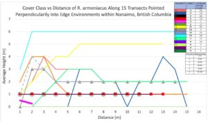
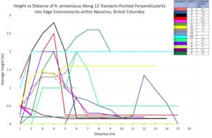
I ended up organizing my data into two graphs containing dependent variables of cover class and average height, and then distance along the transect in meters was the independent variable for each plot. Since I had 15 transects with a maximum of 15 1 m2 quadrats along each transect. My data lined up nicely using distance on the x-axis, but I had to use 15 separate colors, and it took some time to organize the colors and create a legend. One interesting observation from plotting the data was noticing how pervasive Himalayan Blackberry is around Nanaimo. I also noticed how spikes in data occurred around my perceived edge environment in most transects.

mean average height and cove class of R. armeniacus was 0.9 m and 2.09 respectively across all transects. I also saw minimum values of 0 for height and cover class and maximums of 2 m and 6 (95 – 100%). Median values across all 15 transects were also 0.7 m and 1.7 (19%).

In hindsight, I would have chosen 5 to 10 plots along slopes with different aspects and incorporated stand direction into my hypothesis. I also did all of my samplings on the same day so growth was similar across the field site, but if I did the project again I would organize another sampling day a month later.


Post 2: Sources of Scientific Information

User:  | Open Learning Faculty Member: 


A. The source of scientific information is a book entitled Practical Field Ecology: A Project Guide.

Wheater. C , Bell. James, Cook. Penny. (2011). Practical Field Ecology: A Project Guide. Wiley-Blackwell. West Sussex, UK.

B. The source is academic, non-peer reviewed material.

C. Following the tutorial for this module: ‘How to Evaluate Sources of Scientific Information’,  The first step is determining if the material is academic. To determine this, the tutorial has 3 criteria, all must be true. 1) the source must be written by experts in their field. 2) the source must have in text citations. And 3) The source must have a reference or bibliography section.

It is written by 3 authors who are each experts in their respective fields. At the time the book was published, Wheater worked in the department of Environmental and Geographical Sciences at Manchester Metropolitan University; Bell specialized in Plant and Invertebrate Ecology with Rothamsted Research in the UK; and Cook worked in the Faculty of Health and Applied Sciences at Liverpool John Moores University.  The book contains in text citations throughout and has a references section at the back. These three qualities make the book an academic source.

The next question to ask according to the tutorial is: was the material peer reviewed?

The acknowledgements section references many people who assisted in the writing of the book or participated in the required research in some way. However, there is no indication that it was peer reviewed with the possibility of being rejected prior to publication. The publisher does not claim that the book is peer reviewed either. The above points indicate the book is non-peer reviewed.

If the material were peer-reviewed, then the type of peer-reviewed material – research or review could be determined. As the source was not peer-reviewed, it cannot be research or review material.

Post 1: Observations

User:  | Open Learning Faculty Member: 


Site description:

The observation site (The Site) is located at King Street East and Bond Street on the Harmony Creek trail in Oshawa, Ontario. The site is located in an urbanized park with an engineered flood plain and built habitat. The site extends approximately 40 – 50 metres from the harmony creek (which runs north south along the west boundary of the site) on the west to the guard rail of Bond Street on the east. The site follows the creek for approximately 80 metres from a tunnel where Harmony creek passes below King Street in the south to a park bench at the north boundary.

The east creek bank is vegetated with trees, flowering plants and small shrubs. These plants, trees, and shrubs extend from the creek bank, approximately 5 metres to the Harmony Creek Trail – which is paved with asphalt. On the opposite side of the trail (east side), the flood plain is vegetated with manicured grass for approximately 15 – 20 metres. To the east of this grass is a slope that forms the upper boundary of the flood plain. This slope is vegetated with tall grasses, flowering plants and several mature trees.

Time: 4:15 pm. August 9, 2020. Mid-late summer.

Weather:

Partially cloudy. Winds 20 km SSW. 27 degrees Celsius.

Observations:

  • A construction site is set up to the south of the observation area. The path under King street is closed with fencing.
  • Crickets audible in the vegetation near the creek at the south end.
  • Grass is dry and brown to the east of the path.
  • House sparrow observed on the path. It is flying back and forth between from shrubs and the asphalt. Shrubs have grape vines in them.
  • Creek is running calm and clear. No fish observed. No odours or sheens observed. The construction team has installed some netting in the creek.
  • Grassy area on the slope to the east has Dog Strangling Vine growing on it. Vine looks de hydrated. Leaves are shriveled.
  • Monarch butterfly observed flying through the area. No milkweed observed during inspection.

Questions:

  1. What avian species frequent the area?
  2. Is the dog strangling vine spreading? The vines looked to be stressed. Are they producing seeds?
  3. The creek runs through an urbanized area with significant human impact, are any fish species present? Are there any species that run upstream to spawn in the fall at this location?

photos aug 9

Blog Post 5: Design reflections

User:  | Open Learning Faculty Member: 


I did have some difficulties implementing my strategy. Randomly sampling made it hard to select which plant to measure when they were not as abundant in some areas. As well, trying to get an accurate representation from one plant branch of the plant became very challenging. The data was surprising because the plant heights between the two transects looked very different but ended up being very similar.

I will continue collecting my data with the same sampling method (random) with some changes. My data will be continued to be collected at random but i will measure several branches of each plant to average the height for each sample.

Blog Post 4: Sampling Strategies

User:  | Open Learning Faculty Member: 


% error of area densities for systematic, random and haphazard sampling types in the Synder-Middlesworth Natural Area:

Systematic common species % error:

Eastern Hemlock: 20% error

Sweet Birch: 9.8% error

Systematic rare species % error:

Striped Maple: 18.9%

White Pine: 48.8%

Random common species % error:

Eastern Hemlock: 31.7%

Sweet Birch: 14.9%

Random rare species % error:

Striped Maple: 281.1%

White Pine: 50%

Haphazard common species % error:

Eastern Hemlock: 43.9%

Sweet Birch: 53.2%

Haphazard rare species % error:

Striped Maple: 151.4%

White Pine: 100%

The systematic sampling had the lowest sample time with 12hrs 4mins. It was also the most accurate for both common and rare species. Next was random sampling that would take approximately 12hrs 53mins. The slowest and least accurate was the haphazard sampling method at 13hrs 11mins. The results overall seemed to be more accurate throughout all three sampling techniques in the more abundant species such as Eastern Hemlock and Sweet Birch. As well, the overall most accurate sampling method appears to be the systematic method.

Post 3: Ongoing Field Observations

User:  | Open Learning Faculty Member: 


I plan on studying Arctostaphylos uva-ursi (Kinnikinnick).

Hypothesis: Overhead plant life will negatively effect the height of kinnikinnick.

Prediction: Plant height will decrease under layers of vegetation

Response variable: Kinnikinnick

Explanatory variable: Overhead plant life (continuous)

Study is continuous. (Regression approach)

An underlying process that may have caused the observed patterns could be soil type. The open areas had little to no LFH layer and the soil was coarse and very well-drained. The areas of more cover had a little larger of an LFH layer and the soil was less course but still well-drained. This could be the underlying cause of the pigment and growth difference between the two locations.

blog post 3 journal

Post 2: Sources of Scientific Information

User:  | Open Learning Faculty Member: 


The source is on The Effect of NaCl and CMA on the Growth and Morphology of Arctostaphylos uva-ursi (Kinnikinnick).

Young, J. P., Rallings, A., Rutherford, P. M., & Booth, A. L. (2012, January 12). The Effect of NaCl and CMA on the Growth and Morphology of Arctostaphylos uva-ursi (Kinnikinnick). Retrieved August 09, 2020, from https://www.hindawi.com/journals/jb/2012/789879/

This article is academic peer-reviewed research material. The article is formatted as: Abstract, Information, Materials and Methods, Results, Discussion, Acknowledgments and References. This follows the academic scientific article format. I know this is peer-reviewed because at the beginning of the article it states “Academic Editor: Sergi Munne-Bosch”. It also states “Revised 27 Sep 2011. The article is made clear as a research paper when stating materials and methods. Within that section there is a table showing the treatments used in the experiment and a figure showing portions measured of the plant.

Blog Post #6-Data Collection

User:  | Open Learning Faculty Member: 


I have been collecting data for eight weeks over the course of the summer, to coincide with the mating season of frogs and toads on Prince Edward Island. I had four replicates at five locations randomly chosen throughout the South Shore Watershed of Prince Edward Island.

Every two weeks, I would visit five sites after sunset and record their mating calls with my iphone and I also recorded any visual sightings. Prior to the start of my data collection, I placed water temperature loggers at each site, so I was able to record water temperature for each night I was recording the calls. I did not have any trouble sampling, with the exception of mosquitos that attacked me mercilessly. I haven’t noticed any patterns that necessarily agree or disagree with my hypothesis-It is difficult to determine species abundance, especially at night with frogs. I am concerned that my data will show more correlation with mating season than farming. I have already figured on confounding factors based on their actual breeding patterns. I often find myself in these locations during the day, and I am able to see an abundance of leopard frogs, but I don’t hear them at night when recording. Conversely, I never see Spring Peepers, but I record them in abundance.

Blog Post #5-Design Reflections

User:  | Open Learning Faculty Member: 


I have decided to do an abundance study of frogs and toads of PEI and their distance from active farming sites. We only have four frogs-some will say five, but the pickerel frog hasn’t been seen here since 2003, and one toad. The green frog (Rana clamitans), the wood frog (Rana sylvatica), the leopard frog (Rana pipiens), spring peepers (Pseudacris crucifer), and the American toad (Bufo americanus).

My hypothesis is that the species abundance increases as the distance from active farming increases.

I have chosen five sites at random, however, I had to make sure that they had the right environment to support the frogs and toads, so they are all fresh-water riparian sites. I chose those sites and will be measuring the distance to active farming sites through arcGIS. I had some water chemistry analyzed at each of the five sites, however, I only had the funds for one sample at each site, so, depending on their nitrate and phosphorous levels, I will maybe only use this data in my discussion, to hopefully support my hypotheses.

I will drive to each of the five sites during the breeding season at dusk and record their calls for five minutes with my iPhone, then analyze the recordings using their call to identify them and the Abundance Code for Frogs to determine how many are calling:

0 = no amphibians heard
1 = individuals can be counted (no overlapping calls) – estimate of 1-5 individuals calling at site
2 = calls of individuals are distinguishable, but some calls overlap – estimate of 6-10 individuals calling at
site
3 = full chorus, or continuous calls, where individuals cannot be distinguished – estimate of more than
10 individuals calling at the site.

Frogs only call during mating season, so I intend to do 20 site visits (4 nights, at 5 sites) during this time.


Post 5: Design reflections

User:  | Open Learning Faculty Member: 


My initial data collection went well despite the weather factors and wildlife encounters I had to deal with. After many weeks of continuous rain, I was able to go to the site and stake out my study area. I initially was thinking of doing 250m2 based on my google earth location, however, on one side of my study location, there was an active great horned owl’s nest with nestlings that I had to keep distance to minimize stress. On the opposite side perhaps 500m away, a red-tailed hawk pair was nesting and were showing aggressive behavior when in the field. So, I decided to change my study location and study parameters.

With a 100m2, this still allowed me to transect along various zones being tallgrass, cottonwood trees, rocks and floodplain. I removed the upland slope and wetland from my study because of my constraints with the fence-line and wildlife. I added an extra sample to my transect making it 6 quadrats of 0.9144m2  in order to reach the floodplain.

I picked my transect lines at random with a random number generator. My intervals were 15m and sampling at opposite sides to increase randomization. Rather than using the x,y method to go parallel with each zone, I used the x, y method to cross each zone (perpendicular) from the fence-line to the river. I made a mistake by starting my first sampling at 80, 15 instead of sampling at 80, 0. To rectify this issue for my next transect, my options are: create my table with 80, 15 being my starting point; sample the missing quadrat point next time I go back; or select new random numbers and start over.

This will depend if the vegetation has changed and what time of the day I will transect. To improve overall uniformity and reduce bias, I am considering starting over. This wont take much time because I have created waypoints on my GPS of my x,y axis.

Overall, the systematic approach with transects and quadrats was the best method to use to increase my odds of observing absence/presence of ants along the gradient (response variable).