Recent Posts

Blog Post 3: Ongoing Field Observations

User:  | Open Learning Faculty Member: 


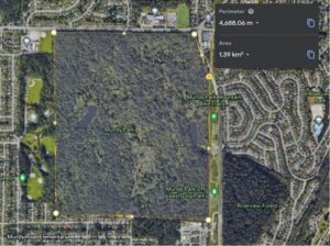
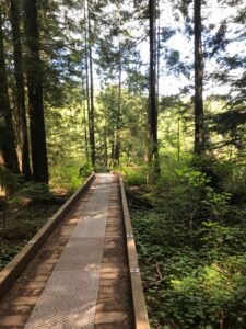
I returned to Edgewater Bar, located in Derby Reach Regional Park in Langley, BC (10 N 527496 5450356). As mentioned previously, the site includes walking trails, a dog park, a picnic area, and fishing along the Fraser River. I arrived to the site at 10:39 am on Sunday, May 2nd, 2021. The weather was a mix of sun and clouds, and the temperature was 13°C. The study area was approximately 400m2 and consisted of the Fraser River (Location 1), the meadow adjacent to the picnic area (Location 2), and the dog park (Location 3). My interest in birds drew my attention back to the American Robins (Turdus migratorius) previously seen foraging for earthworms. I began by observing if the Robins were present or absent in locations 1 through 3.

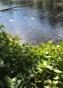
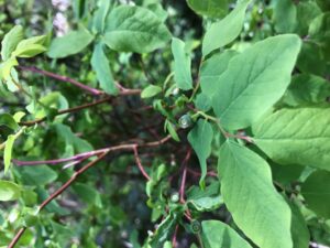
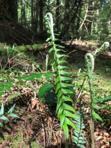
Location 1 – Fraser River: As I approached the river, I could see that the river level was significantly higher than the previous week. Grasses were growing amongst the rocks of the riverbank, which backed onto Western Sword Ferns (Polystichum munitum), Creeping Snowberries (Symphoricarpos mollis), and Himalayan Blackberry (Rubus armeniacus) as the ground changed from rock to soil. No Robins were observed foraging in location 1, likely due to the lack of suitable habitat for earthworms along the rocky riverbank.

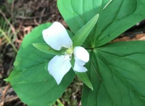
Location 2 – Meadow: As I entered the picnic area, I observed two Robins foraging for earthworms in the meadow. The area consisting of grasses, flowering plants, and trees provided suitable habitat for earthworms due to increased soil moisture. People and their dogs could be seen walking along the trail approximately 15 meters from the foraging Robins. The Robins fledged either when they had enough worms, a loud group walked by, or when a dog entered the meadow. When the Robins had enough worms, they would retreat to the trees, likely where their nest was.

Location 3 – Dog Park: As I proceeded near the edge of the dog park, I observed two Robins foraging. A dog was seen playing fetch with its owner approximately 10 meters away. As the dog ran closer, the Robins fledged to a nearby tree. The Robins would return after the dog left. Shortly after, the gate opened with new dogs entering the park and the Robins fledged. Please note that dogs are only allowed to be off-leash within location 3.

I hypothesize that the length of time a Robin spends foraging in the meadow location will differ from the dog park location. I predict that the length of time a Robin spends foraging in the meadow location will be greater than in the dog park location. I predict this outcome due to the greater number of dogs present within the dog park than the meadow. The response variable for this study is the amount of time a Robin spends foraging at locations 2 or 3, which is continuous, and the explanatory variable for the study will be the presence or absence of dogs which is categorical.

Link to images: https://drive.google.com/drive/folders/1Tg35VPkbahNrzxLXt0PSwr3rMmArTGYU?usp=sharing

Blog Post 1 – Observations

User:  | Open Learning Faculty Member: 


Date/Time:

Visited the site on May 1, 2021, at 16:00.

Weather:

The weather was partly cloudy with no precipitation. The temperature recorded at the site was 17oC. The seasonality is Mid Spring.

Observation Area:

The area that I have chosen to observe is the forested portion of a City park in Coquitlam, BC called Mundy Park. This park is 1.39 km2, has two lakes, is flat and mostly forested.  The park is surrounded by dense suburb developments, and the park trails are a common area for dog walkers and runners.

Figure 1. Satellite View of Mundy Park

Observations:

While walking through the park I noticed that there were different plant species that appear to thrive near the lakes when compared to other regions of the park. My main focus was the abundance of plant species near Mundy lake which is more centrally located in the park and more accessible. The forest seems healthy with few invasive species identified in the central areas of the park. Some of the plant species that I was able to identify are shown in the figures below.

lakeside loop trail
Figure 2. Lakeside Loop Trail

Western trillium
Figure 3. Western trillium

Salal
Figure 4. Salal Near The Lake

Oval-leaf Blueberry
Figure 5. Oval-leaf Blueberry

Western sword fern
Figure 6. Western Sword Fern

Questions

  1. Which areas of the park have the greatest number of Oval-leaf Blueberry and what are the reasons? (sunlight?)
  2. Does proximity to Mundy Lake correlate with a change in the plant species that exist in the area?
  3. Does the proximity to the homes and roads surrounding the park result in a higher number of invasive plant species? (Does the perimeter of the park has more invasive species?)

Blog Post 9: Field Research Reflections

User:  | Open Learning Faculty Member: 


I had originally envisioned random sampling across the entire park. In the end, it was much easier for me to implement my sampling via stratification. For one, the predictor variable I was working with (tree species composition) was fairly well divided into subsections. If I had relied on recording tree species composition for each individual sampling point, I would have had to employ a second sampling unit and a whole secondary methodology to determine which predictor class a given sample fell under. Given my relatively large sample size for the scope of the project (n= 60), it would have taken much longer to collect field data had this been my strategy.

QGIS was instrumental in automating my randomization. I had a few setbacks while trying to transfer data from QGIS to the limited software available for my GPS unit, but overall I think it was worthwhile to employ this strategy. I have used QGIS for a number of applications, including mapping species distributions using herbarium data, but never to implement sampling. It was nice to have an excuse to expand my GIS skillset.

One thing which was challenging about sampling was taking things from the digital realm to the field. From a satellite image or a shapefile it’s impossible to predict which areas will be too dense with brush to reach to sample or where there is standing water (although I didn’t run into the second problem in my data collection). I had a hard time trying not to incorporate subjectivity when I was forced to slightly move my sample site due to unforeseen obstacles. In the end, I decided to move 2m away in a random direction, but its hard to say how random that direction actually is when I have to consciously make the decision to choose a direction. It goes to show that even if you go into the field with fully randomized predetermined sample points, there is always some margin of human subjectivity that gets incorporated into your data.

Lastly, I definitely have a deepened understanding of the development of ecological theory. The pitfalls of trying to observe patterns in nature without accidentally incorporating your own bias toward patterning are prominent and hard to avoid. Like in all science, in ecological theory the importance of building upon previous knowledge and peer review is indispensable in rendering theoretical assertions universally applicable. Without multiple viewpoints, bias cannot be diminished to acceptable levels.

Blog Post 8: Tables and Graphs

User:  | Open Learning Faculty Member: 


For my figure, I used Excel to create a bar chart representing mean percent cover for each of the three stratifications of my study area. I used error bars to depict standard error and tried to keep the visuals as simple and clear as possible.

I am fairly well versed in Excel, so I didn’t run into too much trouble with creating the figure. I was surprised to see my data line up quite well with my prediction. I have yet to conduct statistical analysis of the data, so it remains to be determined if my results are significant.

Blog Post #1 – Dufferin Wetlands

User:  | Open Learning Faculty Member: 


Apr 26 Field Journal

Date/Time: 2021-04-26 at 17:30 hours

Weather: 16oC, partly cloudy

Seasonality: Mid-spring season.

Location: Dufferin Park Wetlands – 1840 Hillside Drive, Kamloops, BC

Designation: City Park


General Description:

Dufferin Park Wetlands is a flat area that is approximately 1900m2. The area was converted into a wetland and designated as a city park in late 2017, and has seen a great deal of development since its creation.

Topography: Dufferin Park Wetlands is located at the base of several hiking trails in the Kenna Cartwright provincial park. Essentially speaking, it is a flat area that is nestled in at the base of a mountain slope. The wetland also bordered by an elementary school, a paved city street, and a set of tennis courts with an attached parking lot.

Vegetation:

The vegetation in this area is primarily comprised of riparian and aquatic wetland type vegetation that transitions into upland vegetation. There are many species of both riparian and aquatic vegetation, which I anticipate to explore in the future.

Observation Questions:

  • Is there a relationship between temperature and species richness/prevalence in this wetland?


    1.  
  • There are many non-aquatic bird species present in the area that appear to be actively competing for territory. What does this type of vegetation offer for these bird species?


    1.  
  • This park is nestled in between a school, tennis courts, a city street, and some provincial park hiking trails. In what ways might these anthropological factors affect this wetland area?


Blog Post 7: Theoretical Perspectives

User:  | Open Learning Faculty Member: 


My project is focused on understanding how site conditions effect the ability of invasive species to colonize new habitat. A species’ “invasiveness” is directly related to their ability to out compete native species. In the Capital Regional District of B.C. , Hedera helix is arguably one of the most detrimental and pervasive alien species. Unlike many other local invasives, H. helix easily penetrates undisturbed or relatively undisturbed habitats, such as the second growth forest of Cuthbert-Holmes Park where I carried out my data collection. In many areas of the C.R.D., native plant diversity is severely reduced as a direct result of H. helix invasion. By deepening our understanding of which sites are most vulnerable to H. helix invasion (in my case, focusing in on a single abiotic factor), we can allocate resources for invasive species control.

Keywords: Hedera helix, site moisture, invasive species, native plant diversity, colonization ability

Blog Post 6: Data Collection

User:  | Open Learning Faculty Member: 


I collected 61 replicates over the three stratified zones. Points were randomly generated using the “Random Points in Polygon” feature in QGIS. First, I determined the area of each of my zones using QGIS. They were as follows:

Alder Zone (zone 1): 7895m2
Grand fir/ Douglas-fir Zone (zone 2): 24239m2
Arbutus/ Garry oak Zone (zone 3): 10932m2

Based on the proportion of the total area that each zone represented, I divided up the 60 replicates to attain the following sampling intensity:

Zone 1: 12 (rounded up from 11.5)
Zone 2: 34
Zone 3: 15

I exported the random points as a GPX file and loaded them onto my GPS. In practice, the sampling strategy worked fairly well. It was difficult to reach some areas due to shrubby undergrowth, but since the areas which were dominated by shrubs lacked H. helix, I was able to visually assess these quadrats. A number of my points landed directly on the trunks of trees, and one landed on a well worn path. For these points, I shifted the sampling over by 2m to the north.

I noticed in my sampling that zone 3 is not entirely contiguous, with some small patches of Douglas-fir dominant stands. Overall, only two points landed in one of these patches, and these data points were not dissimilar from other replicates in the same zone. Since Douglas-fir is able to cope with some level of water stress, I don’t think this is compelling evidence against my stratification. Visually and by touch, the soil is drier in this area, regardless of the presence of arbutus and garry oak.

Reudink, Post 9: Field Research Reflections

User:  | Open Learning Faculty Member: 


Creating a field experiment, carrying it out, analyzing the results, and then interpreting them in a scientific report was an informative experience. Since I have done my entire degree online, I have learned a lot about how different discoveries were scientifically validated but I had not previously had the opportunity to experience this process for myself. I had difficulties in conceiving a good design, initially; however, having a “field expert” on-call, there was always a solution to my issues. One of the largest changes I made was in my sampling design. I went from considering a randomized square plot design to a systematically selected circle plot design. The systematic selection ensured all of my plots were far enough from each other to be independent, while the circle plotting was just plain convenient (i.e., stand in the middle of the circle plot and measure whether specimens are within the radius of the circle).

I have two regrets after completing my study. Firstly, I wish I had the ability to wait for better weather before gathering my data. I am quite certain that the snowy conditions confounded my results. Secondly, I would have liked to fit my data to a model and see whether my correlations were statistically significant. I tried an ANOVA regression and a linear regression; however, the sample size was so small that p values were above 0.6… If I had better statistical know-how, I’m sure I could have found a better model to fit my data to and more accurately measure significance.

Engaging in my own ecological enquiries gives me a deeper appreciation for the work and time that goes into the research that contributes to ecological theory. Just like catching the right camera shot in nature documentaries, collecting good data for ecological science is time-consuming and difficult. This process has also given me an increased sense of curiosity and wonder while I navigate through nature. Who knew science is right around my back door!

Post 2: Sources of Scientific Information

User:  | Open Learning Faculty Member: 


Source of Scientific Information:

  • Vye SR, Dickens S, Adams L, et al. Patterns of abundance across geographical ranges as a predictor for responses to climate change: Evidence from UK rocky shores. Divers Distrib. 2020;26:1357–1365. https://doi. org/10.1111/ddi.13118


Type of information:

  • It can be classified as Academic, peer-reviewed research material.


Evidence to support classification:

  • The paper is written by expert authors that come from different institutions with scientific backgrounds (Bangor University, Newcastle University, University of Liverpool…etc). It also includes in-text citations and has references with all the sources used.
  • The paper was reviewed by three anonymous reviewers that reviewed the manuscript.
  • The paper contains a methods and results section which shows that the researchers conducted field research by collecting data, verifying it, and using statistical analysis to reflect on their results.


Reudink, Post 8: Tables and Graphs

User:  | Open Learning Faculty Member: 


For my project I wanted to see if (a) Populus alba density was correlated with soil moisture content and (b) if P. alba density was different between my measured transects. I compiled my data into a table and also made a few figures. The table was made simply with excel and then I imported the excel sheet into R as a .csv file to make a few figures. I have never been great at using R or excel, but with help of a few YouTube videos and forums I was able to figure out the input required to make the graphs I wanted. My biggest difficulty was ensuring that all of the labels on my graphs were correct.

The outcome of my data was surprising because there was (a) a NEGATIVE correlation between P. alba density and soil moisture content and (b) There was a linear increase in P. alba density from the east transect to the west. This is most surprising because there is a dyke on the west side, so one would think that the soil moisture would be highest closer to the dyke (westward), but the results showed the opposite. This strangeness prompted me to further investigate whether sampling error was a large contributor to this. I am not well-versed in using R to fit data to a model, but I know what normal distributions are supposed to look like on histograms, so I mapped my data onto histograms and analyzed for normality. None was found in my soil samples, so I’m chalking this up to sampling error and would recommend further investigation at a drier time of the year to detect how soil moisture is related to P. alba density. I have attached a word doc of all my figures and tables I will be using for my final report.

Figures and tables for final report